


Differential Equations
#differential equations
#dynamic processes
#mathematical modeling
#educational
#circuit theory
#signal processing
#analog circuits
#simulation
Description: Let us examine the statements that describe the equation. In part (1) of the statement, an unknown function y(t) is added to its derivative y'(t), which is scaled by two multiplier terms, r and c. Differential equations, unlike numerical equations, describe dynamic processes where things are changing. The derivative term y'(t) represents the rate of change in y(t). Consider this system for a moment. Assume that the variable t represents time, although the equation does not necessitate this interpretation. At time zero, the function y(t) equals a; therefore, at that moment, the derivative term y'(t) equals (b - a) / (r * c). Notice that y'(t), which indicates the rate of change in y(t), has its largest value at time zero. Due to the structure of the equation, the value of y'(t) (the rate of change) becomes proportionally smaller as y(t) increases. Eventually, for a very large value of t, the rate of change represented by y'(t) becomes arbitrarily small as y(t) approaches the value of b but never quite reaches it. In simple terms, this equation describes a system in which the rate of change in the value of y(t) depends on the remaining difference between y(t) and b, and as that difference decreases, so does the rate of change. This equation is used to describe many natural processes, including electronic circuits composed of resistors and capacitors (hence the equation's terms r and c), where the voltage across a capacitor changes based on the current flowing through a resistor, and the resistor's current depends on the voltage across the capacitor. It also applies to heat flow between a heat source and a cooler object being heated (such as a pot on a stove), where the temperature of the heated body changes at a rate dependent on the temperature difference between the two bodies. Additionally, it describes the rate of gas flow between two pressure vessels with a constricted passage, where the rate of gas flow depends on the remaining pressure difference, which declines over time. This is not an exhaustive list of the equation's applications. However, the statements regarding a differential equation are just the beginning, and not all differential equations have analytical solutions (expressible as practical functions consisting of standard mathematical operations). Some require numerical methods and are only solvable in an approximate sense. A function that embodies the solution to this differential equation can be utilized to solve real-world problems. An example from electronics involves a circuit consisting of a resistor and a capacitor. At time zero, a switch is closed to connect the circuit to a battery, and an oscilloscope is used to measure the voltage across the capacitor over time.
The described electronic circuit can be represented as an RC (resistor-capacitor) circuit, which is a fundamental configuration in electronics. In this circuit, the resistor (R) and capacitor (C) are connected in series with a voltage source (battery). When the switch is closed at time zero, the capacitor begins to charge through the resistor. The voltage across the capacitor, denoted as V_C(t), increases over time according to the equation derived from the differential equation:
V_C(t) = V_b * (1 - e^(-t/(R*C)))
where V_b is the battery voltage, e is the base of the natural logarithm, and t is the time since the switch was closed. This equation reflects that the voltage across the capacitor approaches the battery voltage asymptotically as time progresses.
The time constant τ of the circuit is defined as τ = R * C, which indicates the time it takes for the voltage across the capacitor to reach approximately 63.2% of its final value (V_b). The behavior of the circuit can be observed on an oscilloscope, where the exponential rise in voltage can be visualized, demonstrating the fundamental principles of charging in an RC circuit.
This RC circuit model can be applied to various practical scenarios, including signal processing, timing applications, and filtering, showcasing the versatility and significance of differential equations in understanding and designing electronic systems.Let`s examine the statements that describe the equation. In part (1) of the statement, we see that an unknown function y(t) is added to its derivative y`(t), which is scaled by two multiplier terms r and c. Remember about differential equations that, unlike numerical equations, they describe dynamic processes ” things are changing.
Remember also that the derivative term y`(t) describes the rate of change in y(t). Please think about this system for a moment. Let`s say that the variable t represents time (although the equation doesn`t require this interpretation). At time zero, the function y(t) equals a, therefore at that moment the derivative term y`(t) is equal to (b - a) / (r * c).
Notice that y`(t), which represents the rate of change in y(t), has its largest value at time zero. Because of how the equation is written, we see that the value of y`(t) (the rate of change) becomes proportionally smaller as y(t) becomes larger. Eventually, for some very large value of t, the rate of change represented by y`(t) becomes arbitrarily small, as y(t) approaches the value of b, but never quite gets there.
Put very simply, this equation describes a system in which the rate of change in the value of y(t) depends on the remaining difference between y(t) and b, and as that difference decreases, so does the rate of change. As it happens, this equation is used to describe many natural processes, among which are: Electronic circuits consisting of resistors and capacitors (hence the equation`s terms r and c), where the voltage on a capacitor changes in a way that depends on the current flowing through a resistor, and the value of the resistor`s current depends on the voltage on the capacitor.
Heat flow between a source of heat energy and a cooler object being heated by it (like a pot on a stove). In such a system, the temperature of the heated body changes at a rate that depends on the remaining difference in temperature between the two bodies.
The rate of gas flow between two pressure vessels with a constricted passage between them. In this system also, the rate of gas flow depends on the remaining pressure difference, and the pressure difference declines over time. This is by no means a comprehensive list of this equation`s applications. But the statements for a differential equation are only the beginning, and not all differential equations have analytical solutions (solutions expressible as a practical function, one consisting of normal mathematical operations).
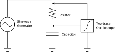
Others require numerical methods and are only soluble in an approximate sense. Okay, we now have a function that embodies the solution to our differential equation. We can use it to solve real-world problems. Here`s an example from a field in which I have spent a lot of time ” electronics. In this experiment, we have an electronic circuit consisting of a resistor and a capacitor. At time zero, we close a switch that connects our circuit to a battery, we then use an oscilloscope to measure the voltage on the capacitor over time (see diagram this page).
The described electronic circuit can be represented as an RC (resistor-capacitor) circuit, which is a fundamental configuration in electronics. In this circuit, the resistor (R) and capacitor (C) are connected in series with a voltage source (battery). When the switch is closed at time zero, the capacitor begins to charge through the resistor. The voltage across the capacitor, denoted as V_C(t), increases over time according to the equation derived from the differential equation:
V_C(t) = V_b * (1 - e^(-t/(R*C)))
where V_b is the battery voltage, e is the base of the natural logarithm, and t is the time since the switch was closed. This equation reflects that the voltage across the capacitor approaches the battery voltage asymptotically as time progresses.
The time constant τ of the circuit is defined as τ = R * C, which indicates the time it takes for the voltage across the capacitor to reach approximately 63.2% of its final value (V_b). The behavior of the circuit can be observed on an oscilloscope, where the exponential rise in voltage can be visualized, demonstrating the fundamental principles of charging in an RC circuit.
This RC circuit model can be applied to various practical scenarios, including signal processing, timing applications, and filtering, showcasing the versatility and significance of differential equations in understanding and designing electronic systems.Let`s examine the statements that describe the equation. In part (1) of the statement, we see that an unknown function y(t) is added to its derivative y`(t), which is scaled by two multiplier terms r and c. Remember about differential equations that, unlike numerical equations, they describe dynamic processes ” things are changing.
Remember also that the derivative term y`(t) describes the rate of change in y(t). Please think about this system for a moment. Let`s say that the variable t represents time (although the equation doesn`t require this interpretation). At time zero, the function y(t) equals a, therefore at that moment the derivative term y`(t) is equal to (b - a) / (r * c).
Notice that y`(t), which represents the rate of change in y(t), has its largest value at time zero. Because of how the equation is written, we see that the value of y`(t) (the rate of change) becomes proportionally smaller as y(t) becomes larger. Eventually, for some very large value of t, the rate of change represented by y`(t) becomes arbitrarily small, as y(t) approaches the value of b, but never quite gets there.
Put very simply, this equation describes a system in which the rate of change in the value of y(t) depends on the remaining difference between y(t) and b, and as that difference decreases, so does the rate of change. As it happens, this equation is used to describe many natural processes, among which are: Electronic circuits consisting of resistors and capacitors (hence the equation`s terms r and c), where the voltage on a capacitor changes in a way that depends on the current flowing through a resistor, and the value of the resistor`s current depends on the voltage on the capacitor.
Heat flow between a source of heat energy and a cooler object being heated by it (like a pot on a stove). In such a system, the temperature of the heated body changes at a rate that depends on the remaining difference in temperature between the two bodies.
The rate of gas flow between two pressure vessels with a constricted passage between them. In this system also, the rate of gas flow depends on the remaining pressure difference, and the pressure difference declines over time. This is by no means a comprehensive list of this equation`s applications. But the statements for a differential equation are only the beginning, and not all differential equations have analytical solutions (solutions expressible as a practical function, one consisting of normal mathematical operations).
Others require numerical methods and are only soluble in an approximate sense. Okay, we now have a function that embodies the solution to our differential equation. We can use it to solve real-world problems. Here`s an example from a field in which I have spent a lot of time ” electronics. In this experiment, we have an electronic circuit consisting of a resistor and a capacitor. At time zero, we close a switch that connects our circuit to a battery, we then use an oscilloscope to measure the voltage on the capacitor over time (see diagram this page).
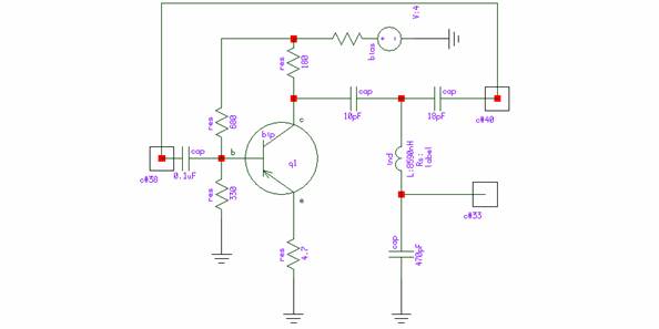
Oscillator Simulation Example Using RINCON
To demonstrate Rincon's capability to simulate autonomous circuits, a one-transistor oscillator utilizing a phase-inverting resonance T-shape LC circuit is considered. The schematic of this simulator is illustrated in Figure 1. The design of the simulator is detailed in reference [2]....
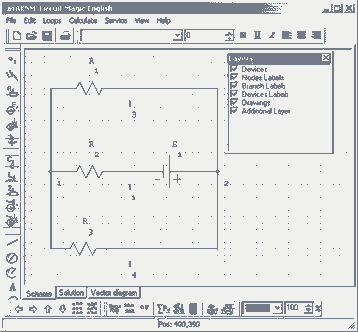
Circuit Magic
Circuit Magic is an electrical circuits simulation program specifically designed for students teaching basics electronics, electrical laws & circuit theory. Unlike many electronic circuit analyzers, Circuit Magic can analyze circuits like a man. Circuits are simulated step by step, using...
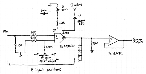
Interpolating Scanner Circuit
This design is for an interpolating scanner, a circuit featuring multiple signal inputs, a control voltage input, and a signal output. The output selectively transitions between inputs, smoothly fading from one to the next as the control voltage increases. A...
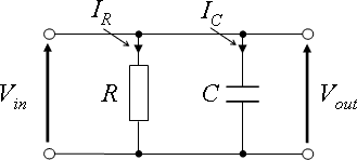
Circuit Theory/All Chapters
This wikibook serves as an introductory text about electric circuits, covering the fundamentals of electric circuit theory, circuit analysis, and circuit design. It is intended as a companion reference for first-year Electrical Engineering undergraduates. Topics include AC and DC circuits,...
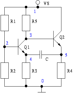
Qualitative Analysis of Analog Circuits
At the beginning of the design process, the designer must determine which circuit structure is appropriate for a specific purpose. During this phase, numerical and symbolic analysis are of limited utility. There are no numerical values available for conventional simulations...
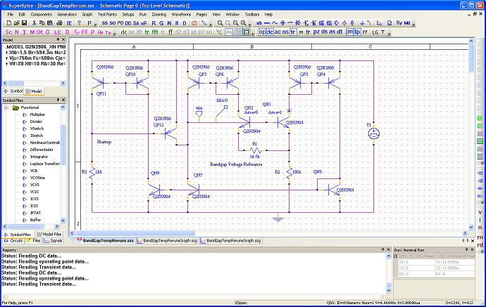
SuperSpice
SuperSpice's philosophy is centered around the edit schematic, run simulation, view waveforms, probe signals, view waveforms, edit schematic cycle. All key issues have been automated. You can effortlessly modify the schematic, rerun and inspect new waveforms without having to reload...