DC Circuit Theory
1. Definition of Direct Current
1.1 Definition of Direct Current
Direct current (DC) is a type of electrical current that flows consistently in one direction, characterized by a constant voltage. This concept is fundamental in understanding various electrical systems and circuits. To grasp the implications of DC, it's essential to differentiate it from alternating current (AC), which fluctuates in direction periodically.
The history of direct current dates back to the 19th century, notably when Thomas Edison championed its use for electrical power distribution. Edison's early systems utilized DC for lighting, marking a pivotal moment in the evolution of electrical engineering and setting the stage for modern electrical infrastructure.
Characteristics of Direct Current
DC circuits possess unique properties that have significant implications in design and application:
- Unidirectional Flow: Unlike AC, the constant flow of electrons in DC does not oscillate, which makes it ideal for many electronic devices.
- Voltage Stability: The steady voltage characteristic of DC ensures that devices requiring a specific voltage can operate consistently without risk of damage.
- Simple Circuit Design: DC circuits are fundamentally simpler than AC circuits, relying on straightforward principles of voltage, current, and resistance.
Mathematical Representation
The fundamental relationship governing direct current is Ohm's Law, represented by the equation:
In the equation above:
- V represents voltage (volts),
- I is the current (amperes), and
- R stands for resistance (ohms).
Within a DC circuit, the current remains constant over time if the resistance remains unchanged, thereby establishing a direct linear relationship between voltage and current. This relationship plays a crucial role in circuit analysis, allowing engineers to predict and control circuit behavior effectively.
Real-World Applications
DC is prevalent in numerous modern applications:
- Electronic Devices: Battery-operated gadgets and smartphones predominantly utilize DC due to their internal circuitry.
- Solar Energy Systems: Photovoltaic cells generate DC power, which can be stored in batteries or converted to AC for use in homes.
- Power Supplies: Many electronic devices require DC power supplies to operate effectively, necessitating the conversion from AC using rectifiers.
Conclusion
Understanding direct current is vital for anyone working in fields related to electrical engineering or electronics. Its distinct characteristics and applications lay the foundation for many technologies in use today. Future innovations will continue to rely on the principles established through the study of DC circuits.
1.2 Voltage, Current, and Resistance
In the landscape of direct current (DC) circuits, voltage, current, and resistance form the trinity that governs the behavior of electrical systems. Understanding the interplay between these three fundamental quantities is essential for engineers and physicists engaged in circuit analysis and design.
Understanding Voltage
Voltage, often referred to as electric potential difference, is the driving force that compels charges to flow within a circuit. Mathematically, it can be described using the equation:
where V represents the voltage (in volts), W is the work done (in joules), and Q is the charge (in coulombs) transferred. This equation underscores the notion that voltage measures the energy transferred per unit charge.
Voltage sources, such as batteries and generators, create potential differences that propel electrons through a conductor. The practical relevance of understanding voltage becomes evident in applications like electronic circuits and power distribution systems, where efficiently managing voltage levels is critical for performance and safety.
Flow of Current
Current, defined as the rate of charge flow, is quantified in amperes (A). It can be mathematically represented as:
Here, I is the current, Q is the total charge flowing, and t represents time. The flow of current is analogous to the flow of water through a pipe, where voltage serves as the pressure that drives the water downstream.
Current exists in two fundamental forms: direct current (DC), where the flow of charge is unidirectional, and alternating current (AC), where the flow periodically reverses direction. In DC applications, understanding current is crucial for circuit design, ensuring components operate within their rated parameters.
The Role of Resistance
Resistance is a measure of the opposition to current flow within a material, influenced by factors including material composition, length, and cross-sectional area. The relationship between voltage, current, and resistance is encapsulated in Ohm’s Law:
In this equation, R is the resistance (in ohms) of the conductor. Ohm’s law serves as the cornerstone for analyzing circuits, enabling the calculation of one parameter when the other two are known. Practically, a thorough grasp of resistance helps engineers select suitable materials and dimensions for conductors, thereby optimizing energy efficiency in various applications.
Summary of Key Relationships
The interconnection between voltage, current, and resistance can be summarized as follows:
- Voltage is the energy per unit charge that drives electrons.
- Current is the rate at which charge flows, impacted by voltage and resistance.
- Resistance opposes current flow and is determined by the material and geometry of the conductor.
Real-World Applications
A robust understanding of voltage, current, and resistance is critical across fields ranging from consumer electronics to electrical engineering. In circuit design, these principles guide the optimization of systems, such as the efficient distribution of power in smart grids or the functioning of low-power devices in Internet of Things (IoT) applications. Engineers harness these relationships to develop safety protocols, ensuring systems remain reliable and effective under varying operational conditions.
1.3 Ohm's Law and its Implications
Ohm's Law stands as one of the fundamental principles in electrical engineering and physics, providing a clear and concise mathematical relationship between voltage, current, and resistance in a direct current (DC) circuit. Mathematically expressed as V = IR, this relationship is pivotal for analyzing and designing electrical circuits.
Understanding the Law
In the equation, V stands for voltage measured in volts (V), I is the current measured in amperes (A), and R represents resistance measured in ohms (Ω). The significance of Ohm's Law lies not only in its simplicity but also in its applicability across a wide spectrum of electrical devices, from basic household appliances to complex industrial systems.
Deriving Ohm's Law
To derive the law, let's start with fundamental definitions:
- Voltage (V): The potential difference that drives the flow of charge carriers.
- Current (I): The rate at which electric charge flows through a conductor.
- Resistance (R): A measure of the opposition to the flow of current.
Through experimental observations, it has been established that for a constant resistance, the current through a conductor between two points is directly proportional to the voltage across the two points. This relationship can be experimentally verified or visualized using a simple circuit where a resistor is connected to a power source:
This fundamental equation leads us to infer that if one variable is known, the others can be calculated easily. For instance, knowing the resistance and the current allows for the calculation of voltage.
Practical Implications of Ohm's Law
The implications of Ohm's Law are profound in both theoretical and practical contexts:
- Circuit Design: Engineers use Ohm's Law extensively when designing circuits by selecting appropriate components to achieve desired voltage and current levels.
- Power Calculations: The power consumed in a circuit can be expressed in terms of voltage and current, leading to the equation P = VI. This highlights the interconnectedness of voltage, current, and power.
- Troubleshooting: Ohm's Law serves as a fundamental tool for electricians and technicians when diagnosing faulty circuits, allowing them to identify issues related to overloads and short circuits.
Real-World Applications
In the modern world, applications of Ohm's Law manifest in numerous technologies:
- Consumer Electronics: Devices like smartphones and laptops utilize the principles of Ohm's Law for battery management systems ensuring efficient energy use.
- Renewable Energy Systems: In systems like solar panels, understanding the workings of DC circuits and the significance of resistance enables better optimization of the energy produced.
- Automated Systems: In robotics and automation, Ohm's Law is critical for controlling servos and motors, ensuring they operate within safe voltage and current limits.
As technology continues to advance, the relevance of Ohm's Law will persist as a cornerstone for understanding and manipulating electrical systems.
2. Resistors: Types and Characteristics
2.1 Resistors: Types and Characteristics
Resistors are fundamental components in DC circuits, serving to limit current flow, divide voltages, and dissipate energy as heat. Their role is crucial in protecting sensitive components and controlling the behavior of electrical networks.
Types of Resistors
Understanding the diverse types of resistors is essential for engineers and researchers alike, as their unique characteristics influence circuit design and performance. Resistors can be categorized based on several criteria, including construction, material, and application.
Fixed Resistors
Fixed resistors maintain a constant resistance value. They are typically made of carbon composition, carbon film, metal film, or wirewound materials.
- Carbon Composition Resistors: These resistors are made from a mixture of carbon and a binding material. They are generally used in low-frequency applications due to their noise generation and tolerance variability.
- Metal Film Resistors: Known for their superior stability and low noise, metal film resistors are ideal for precision applications. They provide better temperature coefficients and lower tolerances.
- Wirewound Resistors: These resistors consist of a wire wound around an insulating core and are useful in high-power applications due to their excellent heat dissipation properties.
Variable Resistors
Variable resistors, also known as potentiometers or rheostats, allow the resistance to be adjusted manually. They are used for applications such as volume control in audio equipment or adjusting levels in analog circuits. The mechanism typically involves a wiper that slides over a resistive element, changing the resistance value depending on the position.
Characteristics of Resistors
The selection and application of resistors depend heavily on their characteristics, which include resistance value, tolerance, temperature coefficient, and power rating.
Resistance Value
The resistance value, measured in ohms (Ω), determines how much a resistor opposes the flow of current. In DC circuits, Ohm's Law, expressed as:
where V is the voltage across the resistor, I is the current flowing through it, and R is the resistance, governs the relationship between these quantities.
Tolerance
Tolerance indicates how much a resistor's actual resistance can deviate from its specified value, expressed as a percentage. For example, a resistor with a value of 100 Ω and a tolerance of ±5% can range from 95 Ω to 105 Ω. Tolerance is crucial in precision applications where slight deviations can affect circuit performance.
Temperature Coefficient
The temperature coefficient specifies the change in resistance with temperature variation, typically expressed in ppm/°C (parts per million per degree Celsius). A low temperature coefficient ensures that the resistor maintains its performance across varying environmental conditions, which is key for stability in sensitive circuits.
Power Rating
The power rating, measured in watts (W), indicates the maximum power a resistor can safely dissipate without overheating. The power dissipated by a resistor in a circuit can be calculated using:
or
where P is power, I is current, and V is voltage. Selecting a resistor with an adequate power rating is imperative for avoiding failure and maintaining circuit integrity.
Practical Applications
Resistors are ubiquitous in electronic devices. For instance, in voltage divider circuits, resistors are utilized to produce a specific output voltage. In filter circuits, they interact with capacitors and inductors to shape signal characteristics. Moreover, in sensor applications, resistors are essential for setting thresholds and calibrating responses.
As technology advances, new materials and designs, such as thin-film and thick-film resistors, continue to emerge, offering improved performance and miniaturization potential. Understanding the implications of resistor types and their characteristics is imperative for advancing reliable and efficient electrical systems.
2.2 Capacitors: Operational Principles
Capacitors are essential components in electrical circuits, serving various crucial roles ranging from energy storage to filtering. Understanding their operational principles provides insights into their functionality and the myriad applications they support across different fields of engineering and physics.
Basic Concept of Capacitance
At its core, capacitance is the ability of a capacitor to store electric charge. Defined mathematically, the capacitance \(C\) of a capacitor is given by the ratio of the electric charge \(Q\) stored to the voltage \(V\) across its terminals:
Capacitance is measured in farads (F), where 1 farad corresponds to a capacitor that stores 1 coulomb of charge at 1 volt. Although practical capacitors typically have capacitance values in microfarads (µF) or picofarads (pF), understanding the fundamental definition is crucial.
Construction and Operation
Capacitors comprise two conductive plates separated by an insulating material known as the dielectric. The dielectric material can significantly influence the capacitor's performance, with common materials including air, ceramic, paper, and electrolytic substances. When a voltage is applied across the plates, an electric field is established, allowing the capacitor to store energy in the form of an electric field.
Charging and Discharging Dynamics
The behavior of a capacitor during charging and discharging is critical to understanding its application in circuits. When connected to a voltage source, the charging process can be characterized by the equation for current \(I\) as a function of time \(t\):
As the capacitor charges, the voltage across it increases, impacting the current flowing into the capacitor. Eventually, the capacitor reaches its maximum charge, effectively acting as an open circuit when fully charged. Conversely, upon discharging, it releases stored energy back into the circuit, typically characterized by an exponential decay of voltage and current, which can be modeled by the time constant \(τ\):
Here, \(R\) represents the total resistance in the circuit. The exponential decay can be described by the equation:
where \(V_0\) is the initial voltage across the capacitor at \(t = 0\). Understanding this behavior is essential when designing timing circuits or filtering applications.
Real-World Applications
Capacitors are ubiquitous in electronic devices, serving functions such as:
- Energy Storage: Used in power supply systems to smooth out voltage fluctuations.
- Filtering: In audio systems and radio transmitters, capacitors can filter unwanted frequencies.
- Timing Circuits: In combination with resistors, capacitors are used in oscillators and timers.
These applications demonstrate the versatility of capacitors in powering modern technology, from simple devices to complex systems.
Conclusion
In summary, understanding capacitors and their operational principles is a fundamental aspect of DC Circuit Theory. With their ability to store and release energy, their applications in filtering, timing, and power management highlight their critical role in modern electrical engineering. The dynamics of charging and discharging further open avenues for innovation in circuit design, leading to more efficient and effective electronic devices.
2.3 Inductors: Effect on DC Circuits
Inductors play a pivotal role in the behavior of DC circuits, although their effects are often less prominent than in AC systems. Understanding how inductors interact with direct current can reveal significant insights into circuit performance, especially during transient states, which are critical in applications such as power supplies, motors, and signal filtering.
What is an Inductor? An inductor, or coil, is a passive electronic component that stores energy in a magnetic field when electrical current passes through it. The fundamental property of an inductor is its inductance, measured in henries (H). This inductance determines how much voltage is induced across the inductor in response to a change in current.
Inductor Behavior in DC Circuits
When connected to a DC source, the initial response of an inductor is to resist changes in current. According to Lenz's Law, the inductor generates an electromotive force (EMF) opposite to the change in current, which leads to interesting dynamics in the circuit. The responses can be characterized in two main phases: the transient phase and steady-state phase.
Transient Phase
Upon switching on a DC current, the inductor experiences a change in magnetic field, thereby generating voltage. The governing equation for current through an inductor is given by:
Where:
- VL is the induced voltage across the inductor in volts,
- L is the inductance in henries,
- di/dt is the rate of change of current in amperes per second.
This means that the voltage across the inductor will be highest when the current changes rapidly (i.e., when the switch is first closed). As time progresses and the switch remains closed, the current stabilizes, leading to zero voltage across the inductor under steady-state conditions.
In this equation:
- I(t) is the current at time t,
- I0 is the final steady-state current,
- R is the series resistance in ohms,
- e is Euler's number, approximately equal to 2.71828.
Steady-State Phase
Once the circuit reaches a stable condition, the inductor can be viewed as a short circuit for DC current. This is because, in steady-state, there is no change in current, leading to no induced voltage:
These properties are essential when designing circuits that require inductors, such as smoothing out the current fluctuations in power supplies or inductive loads in motor control applications.
Practical Applications of Inductors in DC Circuits
The behavior of inductors in DC circuits is utilized in various real-world applications:
- Switching Power Supplies: Inductors are used to store energy temporarily and release it as needed, improving operational efficiency.
- Voltage Regulation: Inductors help minimize ripples in output voltage, resulting in a steady DC supply.
- High-Frequency Applications: Inductors filter out unwanted high-frequency signals, ensuring that only desired frequencies pass through.
By grasping the principles of how inductors function in DC circuits, engineers and designers can leverage these components to create efficient and reliable electronic systems.
3. Series vs. Parallel Circuits
3.1 Series vs. Parallel Circuits
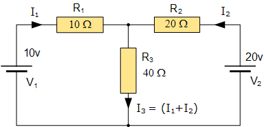
Understanding the principles of series and parallel circuits is fundamental to grasping the more complex behaviors encountered in DC circuit theory. These configurations dictate electrical flow, impact the total resistance, and largely affect voltage distribution across components. While they are conceptually straightforward, their implications can significantly alter circuit performance in practical applications, such as in network design or the use of microcontrollers.Basic Definitions and Characteristics
In electrical engineering, series circuits and parallel circuits represent two fundamental ways of connecting components. Series Circuit: In a series configuration, components are connected end-to-end in a single path for current to flow. Thus, the same amount of current flows through each component, and the total voltage across the circuit is the sum of the individual voltage drops across each resistor. Parallel Circuit: Conversely, a parallel configuration allows components to be connected across the same two nodes, creating multiple paths for the current to flow. This results in each component experiencing the same voltage, while the total current is the sum of the currents flowing through each parallel branch. A diagram can help illuminate these configurations. In a typical series circuit, resistors \( R_1 \), \( R_2 \), and \( R_3 \) are aligned in a single path. In a parallel circuit, the same resistors are connected between two voltage sources, effectively branching out from the source.Mathematical Analysis of Series and Parallel Circuits
To quantitatively evaluate these circuits, we can derive some key equations: 1. Series Resistance: The total resistance \( R_T \) in a series circuit is simply the sum of the individual resistances:Practical Applications and Distinctions
The importance of selecting whether to implement a series or parallel circuit cannot be understated in both theoretical and practical contexts. Series Circuits: - Advantages: - Simple design. - Predictable voltage drop across components. - Easy to understand and troubleshoot. - Applications: Commonly found in string lights where if one bulb blows, the entire string goes out, demonstrating the dependency of components upon one another. Parallel Circuits: - Advantages: - Independent operation of each component. - Greater reliability since the failure of one path does not halt the other operations. - Applications: Used in household wiring, where appliances can operate independently without affecting one another's performance. Understanding these distinctions and applications enhances one's ability to design and analyze electrical systems effectively, optimizing for desired performance outcomes while balancing the trade-offs effectively. The analysis becomes even more salient as circuits grow in complexity, often incorporating both series and parallel components.3.2 Kirchhoff's Laws: Voltage and Current
The analysis of direct current (DC) circuits is profoundly rooted in two foundational principles, known as Kirchhoff's Laws. Established by the German physicist Gustav Kirchhoff in the mid-19th century, these laws provide a systematic method for analyzing complex circuits involving resistors, capacitors, and other components. Understanding these principles is crucial for engineers and physicists alike, as they serve not only as a basis for theoretical circuit design but also for practical applications in various technologies, from simple circuits to sophisticated electronic devices.
At the core of Kirchhoff's approach are the laws governing current and voltage at nodes and loops within a circuit. These laws facilitate the analysis and understanding of electric circuits, allowing for predictions about the behavior of electrical systems under various conditions.
3.2.1 Kirchhoff's Current Law (KCL)
KCL states that the total current entering a junction or node must equal the total current leaving that node. This law is derived from the principle of conservation of electric charge, which asserts that charge cannot be created or destroyed. Mathematically, this can be expressed as:
To visualize KCL, consider a node with three incoming currents \(I_1\), \(I_2\), and \(I_3\) and two outgoing currents \(I_4\) and \(I_5\). The algebraic sum at the node must adhere to KCL:
3.2.2 Kirchhoff's Voltage Law (KVL)
KVL complements KCL and articulates that the sum of the electrical potential differences (voltage) around any closed loop within a circuit must be zero. This stipulation is rooted in the conservation of energy principle, indicating that energy supplied by sources in the loop must account for energy losses through resistive components. Mathematically, KVL can be expressed as:
In practical terms, this can be represented in a simple circuit with a single loop. If there are voltages \(V_1\), \(V_2\) (supplied by sources), and voltage drops \(V_3\) and \(V_4\) across resistors, KVL leads us to:
3.2.3 Application of Kirchhoff's Laws in Circuit Analysis
Both KCL and KVL are instrumental in circuit analysis techniques such as nodal analysis and mesh analysis. Nodal analysis employs KCL to solve for unknown voltages at circuit nodes, while mesh analysis utilizes KVL to ascertain currents in defined loops. These methodologies are widely applicable in fields such as telecommunications, control systems, and power distribution, facilitating the design and optimization of circuits.
Furthermore, Kirchhoff's Laws are foundational in the development of simulation software such as SPICE, which allows engineers to model and analyze circuit behavior under an array of conditions. This applicability underscores the significance of these laws in both theoretical studies and practical engineering endeavors.
In contemporary applications, an understanding of Kirchhoff's Laws is vital for addressing challenges in circuit stability, efficiency, and power management, especially in integrated circuits and advanced electronic systems.
3.3 Thevenin's and Norton's Theorems
In analyzing complex circuits, engineers often encounter the challenge of simplifying the analysis process while preserving essential circuit characteristics. Here, Thevenin's and Norton's theorems play critical roles by allowing the conversion of complicated networks into simpler equivalent circuits.
Thevenin's Theorem
Thevenin's Theorem states that any linear electrical network with voltage sources and resistors can be transformed into a single voltage source (Thevenin voltage, V_th) in series with a single resistor (Thevenin resistance, R_th). This simplification is invaluable when analyzing the power delivered to a load. The practical relevance of Thevenin’s theorem emerges in various fields, from power system analysis to electronics design.
The steps to apply Thevenin's theorem are as follows:
- Identify the portion of the circuit you wish to simplify.
- Remove the load resistor across which you want to find the output voltage.
- Calculate the Thevenin voltage (V_th) by finding the open-circuit voltage at the terminals.
- Calculate the Thevenin resistance (R_th) by deactivating all independent sources (replace voltage sources with short circuits and current sources with open circuits) and finding the equivalent resistance at the terminals.
The resulting equivalent circuit can be visualized succinctly as:
Where R_L is the load resistance connected to the simplified circuit, thus facilitating easier calculations of current, voltage, and power.
Norton's Theorem
In contrast, Norton’s Theorem posits that any linear circuit can be represented as an equivalent current source (Norton current, I_n) in parallel with a single resistor (Norton resistance, R_n). The advantage of Norton’s theorem lies in its ability to analyze circuits that require a current across multiple paths.
The steps for applying Norton’s theorem are similar and include:
- Select the part of the circuit for analysis and remove the load resistor.
- Calculate the Norton current (I_n) by finding the short-circuit current between the terminals.
- Determine the Norton resistance (R_n) by deactivating independent sources as described earlier.
With the circuit transformed, we can express the output voltage as:
Interrelationship between Thevenin's and Norton's Theorems
Thevenin's and Norton's theorems are closely related. Each theorem can be derived from the other, characterized by the relationships:
- V_th = I_n \cdot R_n
- R_th = R_n
Thus, the equivalent voltage and current sources can seamlessly interchange based on the load requirements. This means that, depending on circuit configurations and analysis goals, either theorem can be practically applied to reduce complexity while preserving the circuit’s behavior.
In practical applications, engineers may utilize software tools that implement these theorems to simulate circuit behavior quickly. Applications range from the design of amplifiers in audio equipment to power management in renewable energy systems.
4. Calculating Power: Basic Formulas
4.1 Calculating Power: Basic Formulas
Understanding the concept of power in DC circuits is essential for engineers and physicists as it directly affects the functionality and efficiency of electrical systems. Power is the rate at which energy is consumed or transferred, and in the realm of direct current (DC) circuits, calculating power involves a straightforward application of Ohm's law and the relationships between current, voltage, and resistance. This section will delve into the foundational formulas for power calculation, incorporating practical implications and derivations for a comprehensive understanding.
Foundational Formulas
The fundamental relation for electrical power in DC circuits can be summarized using three key formulas, each providing a different perspective on the interacting parameters of voltage, current, and resistance. The power \( P \) in watts (W) can be calculated using the following equations:
Here, \( V \) stands for voltage in volts (V), and \( I \) represents current in amperes (A). This equation is immensely practical; it shows how power increases as either voltage or current increases.
Deriving Alternative Forms
In addition to \( P = VI \), we can derive two alternative expressions by employing Ohm's law, which states \( V = IR \), where \( R \) is the resistance measured in ohms (Ω). Using this relationship, we can substitute \( V \) into our original equation:
This equation indicates that power is also proportional to the square of the current multiplied by the resistance. Thus, for situations where current is easy to measure, this relationship becomes particularly useful.
Conversely, if we manipulate Ohm's law to express current in terms of voltage and resistance, we obtain:
By substituting this expression into the power equation \( P = VI \), we arrive at another important form:
This equation shows that power can also be calculated as the square of the voltage divided by the resistance, which is particularly handy when voltage is more accessible than current in a measurement setup.
Practical Applications
These foundational formulas facilitate various practical applications in electrical engineering. For instance, they are fundamental in the sizing of components in circuit design to ensure that resistances, currents, and voltages are optimal for performance while maximizing efficiency and minimizing heat generation. In power systems analysis, these formulas are employed to calculate the power dissipation in resistors, informing the selection of materials and designs for devices ranging from small electronics to large industrial machines.
Moreover, circuit simulation software often integrates these calculations, allowing for rapid assessments of circuit performance under varying conditions. Understanding these relationships is crucial when designing circuits that require specific power handling capabilities, such as in renewable energy systems or traditional electrical grid applications.
In summary, the versatility and significance of power formulas can not be overstated in DC circuit theory. Mastery of these basic equations forms the foundation for tackling more complex analyses in both theoretical research and practical engineering solutions. The continuous exploration of these concepts leads to advancements in technology and improved energy efficiency across various applications.
4.2 Power Dissipation in Resistors
Understanding the principles of power dissipation in resistors is fundamental for engineers and physicists alike, as it lays the groundwork for analyzing circuit performance. When a current flows through a resistor, electrical energy is converted into thermal energy, leading to power dissipation. This section will explore the underlying principles of this process, the associated equations, and its implications in real-world applications.Power Dissipation Fundamentals
When discussing power in electrical circuits, it is essential to recognize that power dissipation refers to the energy converted into heat as electrical energy flows through resistive elements. In ohmic materials, where resistance \( R \) is constant with respect to current, Ohm's law provides the framework:Practical Relevance of Power Dissipation
The concept of power dissipation is not purely theoretical; it plays a critical role in several practical applications:- Component Selection: Engineers must choose resistors with appropriate power ratings to prevent overheating and possible device failure. This power rating is typically provided in datasheets.
- Heat Management: In circuits where high currents flow, effective cooling methods or the use of heat sinks is necessary to dissipate excess heat and maintain operational integrity.
- Energy Efficiency: Understanding power dissipation helps in optimizing circuits for energy consumption, which is essential in battery-powered devices.