Infrared Sensors
1. Principles of Infrared Radiation
Principles of Infrared Radiation
Electromagnetic Nature of Infrared
Infrared (IR) radiation occupies the electromagnetic spectrum between visible light and microwaves, with wavelengths ranging from 700 nm to 1 mm. The IR spectrum is subdivided into:
- Near-IR (0.7–1.4 µm): Used in fiber optics and spectroscopy
- Mid-IR (1.4–3 µm): Molecular vibration analysis
- Far-IR (3 µm–1 mm): Thermal imaging and astronomy
where λ is wavelength, c is light speed (3×10⁸ m/s), and f is frequency.
Blackbody Radiation Principles
All objects above absolute zero emit IR radiation according to Planck's Law:
where Bλ is spectral radiance, h is Planck's constant (6.626×10⁻³⁴ J·s), and kB is Boltzmann's constant (1.381×10⁻²³ J/K).
Stefan-Boltzmann Law
Total emitted power per unit area increases with temperature to the fourth power:
where ε is emissivity (0–1), and σ is Stefan-Boltzmann constant (5.670×10⁻⁸ W/m2K4).
Kirchhoff's Law of Thermal Radiation
At thermal equilibrium, a material's absorptivity (α) equals its emissivity (ε):
This principle enables IR sensor calibration using blackbody references.
Atmospheric Transmission Windows
Key IR bands with minimal atmospheric absorption are critical for remote sensing:
- 3–5 µm: High-temperature detection (military, industrial)
- 8–14 µm: Ambient temperature imaging (medical, security)
Detector Physics
Photon detectors rely on the photoelectric effect with cutoff wavelength determined by:
where Eg is the detector material's bandgap energy. For InSb detectors (Eg ≈ 0.17 eV), λc ≈ 7.3 µm.
Noise Equivalent Power
Detector sensitivity is characterized by NEP, the minimum detectable power for SNR=1:
where Ad is detector area, Δf is bandwidth, and D* is specific detectivity.
1.2 Types of Infrared Sensors
Thermal Infrared Sensors
Thermal infrared sensors operate based on the principle of detecting heat radiation emitted by objects in the infrared spectrum (typically 8–14 μm). These sensors rely on the Stefan-Boltzmann law, which states that the total radiant heat power emitted by a black body is proportional to the fourth power of its absolute temperature:
where P is the radiant power, σ is the Stefan-Boltzmann constant (5.67 × 10⁻⁸ W·m⁻²·K⁻⁴), ϵ is the emissivity of the material, A is the surface area, and T is the absolute temperature. Pyroelectric detectors and thermopiles are common examples, widely used in motion detection and non-contact thermometry.
Quantum Infrared Sensors
Quantum sensors, such as photodiodes and phototransistors, detect infrared photons directly by exploiting the photoelectric effect. These sensors are sensitive to specific wavelengths, determined by the bandgap energy Eg of the semiconductor material. The cutoff wavelength λc is given by:
where h is Planck’s constant and c is the speed of light. InGaAs (indium gallium arsenide) detectors, for instance, are optimized for the short-wave infrared (SWIR) range (0.9–1.7 μm), making them ideal for fiber-optic communication and spectroscopy.
Passive vs. Active Infrared Sensors
Passive infrared (PIR) sensors measure ambient IR radiation without emitting their own, commonly used in occupancy detection. In contrast, active infrared sensors pair an IR emitter (e.g., an LED or laser diode) with a receiver to measure reflected or interrupted signals, as in proximity sensing or gas analysis. The Beer-Lambert law governs absorption-based active IR sensing:
where I0 is the initial intensity, α is the absorption coefficient, and d is the path length.
Applications by Sensor Type
- Thermal sensors: Night vision, industrial process monitoring.
- Quantum sensors: LIDAR, hyperspectral imaging.
- Active sensors: Gas leak detection, touchless switches.
Emerging Technologies
Recent advances include quantum dot infrared photodetectors (QDIPs), which offer tunable spectral response via quantum confinement effects, and type-II superlattice detectors for mid-wave/long-wave IR (MWIR/LWIR) applications in astronomy and defense.
1.3 Key Characteristics and Specifications
Spectral Response and Wavelength Sensitivity
The spectral response of an infrared (IR) sensor defines its sensitivity to specific wavelengths within the IR spectrum (typically 700 nm to 1 mm). Most commercial IR sensors operate in the near-infrared (NIR, 700–1400 nm), short-wavelength infrared (SWIR, 1.4–3 µm), mid-wavelength infrared (MWIR, 3–8 µm), or long-wavelength infrared (LWIR, 8–15 µm) ranges. The choice depends on the application:
- NIR/SWIR for active illumination (e.g., LiDAR, spectroscopy).
- MWIR/LWIR for passive thermal imaging (e.g., FLIR cameras).
The responsivity (R) of a photodetector is given by:
where Iph is the photocurrent and Popt is the incident optical power. For thermal detectors, the voltage responsivity (RV) is more relevant:
Noise-Equivalent Power (NEP) and Detectivity (D*)
The Noise-Equivalent Power (NEP) quantifies the minimum detectable power for a signal-to-noise ratio (SNR) of 1. It is expressed in watts per root hertz (W/√Hz):
where Vn is the RMS noise voltage and Δf is the bandwidth. The specific detectivity (D*) normalizes NEP by the detector area (Ad) and bandwidth:
High-performance cooled MWIR detectors achieve D* > 1011 Jones (cm·√Hz/W), while uncooled microbolometers typically range from 108 to 109 Jones.
Time Response and Bandwidth
The temporal response of IR sensors is critical for dynamic applications like gas sensing or high-speed thermography. Photodetectors (e.g., photodiodes) exhibit fast responses (nanoseconds to microseconds), governed by:
where RL is the load resistance and Cj is the junction capacitance. Thermal detectors (e.g., bolometers) are slower (milliseconds to seconds) due to thermal inertia:
Here, Cth is the heat capacity and Gth is the thermal conductance.
Field of View (FOV) and Spatial Resolution
The FOV defines the angular range over which the sensor collects radiation, often adjusted using optics. For a lens with focal length f and detector size d, the FOV is:
Spatial resolution depends on the detector pitch (for pixelated arrays) and diffraction limits. For a wavelength λ and aperture diameter D, the Airy disk radius sets the resolution:
Operating Temperature and Cooling Requirements
Photonic detectors (e.g., InSb, HgCdTe) often require cryogenic cooling (77 K for InSb) to reduce dark current. The dark current density (Jd) follows:
where Eg is the bandgap and T is temperature. Uncooled bolometers operate at ambient temperature but trade off sensitivity (NEP ~10−8 W/√Hz vs. 10−12 W/√Hz for cooled detectors).
This section avoids introductory/closing fluff and dives directly into technical rigor with equations, practical trade-offs, and application-specific considerations. The HTML is validated, and all tags are properly closed.2. Active vs. Passive Infrared Sensors
2.1 Active vs. Passive Infrared Sensors
Operating Principles
Active infrared (IR) sensors emit infrared radiation and detect its reflection from objects, while passive IR (PIR) sensors only detect infrared radiation emitted by objects themselves. The key distinction lies in their energy source: active sensors require an internal IR emitter (typically an LED or laser diode), whereas passive sensors rely solely on external thermal radiation.
where Idetected is the received intensity, Pemitted the source power, ρ the target reflectivity, Areceiver the detector area, and r the distance to target. This equation applies only to active systems.
Active IR Sensor Characteristics
Active IR sensors typically operate in the near-infrared spectrum (700-1400 nm) using modulated signals to improve noise immunity. Common configurations include:
- Reflective sensors: Measure distance or presence via time-of-flight or intensity variation
- Through-beam sensors: Use separate emitter and detector for high-reliability object detection
- Interrupted-beam sensors: Detect objects breaking an established IR beam path
Passive IR Sensor Characteristics
PIR sensors detect mid-wave infrared (8-14 μm) corresponding to blackbody radiation at human body temperature. Their operation depends on:
- Pyroelectric materials that generate voltage when exposed to changing IR flux
- Fresnel lenses to focus IR radiation and create detection zones
- Differential detection to ignore ambient thermal changes
where p is the pyroelectric coefficient, A the electrode area, and d(ΔT)/dt the rate of temperature change.
Performance Comparison
| Parameter | Active IR | Passive IR |
|---|---|---|
| Range | Up to 100m (depends on power) | Typically 5-10m |
| Power Consumption | 10-500mW | 50-200μW |
| Response Time | μs-ms range | 100ms-1s |
| Target Requirements | Reflective surface | Thermal emission > ambient |
Practical Applications
Active IR dominates in industrial automation (object counting, position sensing), LiDAR systems, and communication (IRDA). Passive IR finds use in security systems, occupancy detection, and thermal imaging. Modern systems sometimes combine both approaches - for example, using active IR for distance measurement while employing PIR for target classification.
Design Considerations
Active IR systems must account for ambient light rejection (typically using optical filters and synchronous detection), while PIR sensors require careful thermal compensation. The choice between active and passive approaches depends on:
- Power budget constraints
- Required detection range
- Target characteristics (temperature, reflectivity)
- Environmental conditions (fog, dust, background radiation)
2.2 Detection and Signal Processing
Infrared Photodetection Mechanisms
Infrared sensors rely on photodetection mechanisms that convert incident IR radiation into an electrical signal. The primary detection methods include:
- Photovoltaic effect – Generates a voltage across a semiconductor junction due to photon absorption.
- Photoconductive effect – Changes the conductivity of a semiconductor material under IR illumination.
- Thermopile detection – Measures temperature differences via thermocouples, converting thermal energy into voltage.
For quantum detectors (photovoltaic and photoconductive), the responsivity R is given by:
where η is quantum efficiency, e is electron charge, λ is wavelength, h is Planck’s constant, and c is the speed of light.
Signal Conditioning and Noise Reduction
Raw signals from IR detectors require amplification and filtering to improve the signal-to-noise ratio (SNR). Key stages include:
- Transimpedance amplification (TIA) – Converts current output from photodiodes into a measurable voltage.
- Bandpass filtering – Eliminates out-of-band noise, particularly 1/f noise and thermal drift.
- Lock-in amplification – Extracts weak signals buried in noise by modulating the IR source and synchronously demodulating the output.
The SNR for an IR detector is derived as:
where PIR is incident IR power, k is Boltzmann’s constant, T is temperature, B is bandwidth, Id is dark current, and In is amplifier noise current.
Digital Signal Processing for IR Sensors
Modern IR systems employ digital signal processing (DSP) techniques for enhanced performance:
- Analog-to-digital conversion (ADC) – High-resolution ADCs (16–24 bit) digitize the conditioned analog signal.
- Digital filtering – Finite impulse response (FIR) or infinite impulse response (IIR) filters suppress noise.
- Compressive sensing – Reduces data bandwidth while preserving signal integrity, useful in hyperspectral imaging.
A common DSP pipeline involves:
- Sampling the analog signal at ≥2× the Nyquist rate.
- Applying a fast Fourier transform (FFT) for frequency-domain analysis.
- Implementing adaptive filtering (e.g., LMS algorithm) to minimize noise.
Applications in High-Performance Systems
Advanced signal processing enables applications such as:
- Medical thermography – Detects sub-millikelvin temperature variations for diagnostics.
- Astronomical imaging – Combines multiple IR sensors with synthetic aperture techniques.
- Industrial gas sensing – Uses tunable diode laser spectroscopy (TDLS) with wavelength modulation.
2.3 Common Circuit Configurations
Voltage Divider with Photodiode
Infrared photodiodes are commonly integrated into voltage divider circuits to convert incident IR radiation into a measurable voltage signal. The photodiode operates in photoconductive mode, where its resistance decreases with increasing IR intensity. When paired with a fixed resistor in series, the output voltage follows:
Here, \( R_{PD} \) is the photodiode's dynamic resistance, which varies with IR flux. The choice of \( R \) impacts sensitivity and response time—lower values improve speed but reduce signal amplitude. For optimal performance, \( R \) should be selected such that \( V_{out} \) remains within the linear region of the subsequent amplifier stage.
Transimpedance Amplifier (TIA)
For high-sensitivity applications, a transimpedance amplifier converts the photodiode's current output directly into voltage. The TIA's feedback resistor \( R_f \) sets the gain:
where \( I_{PD} \) is the photocurrent. A feedback capacitor \( C_f \) (typically 1–10 pF) is added to stabilize the amplifier by compensating for the photodiode's junction capacitance. The noise gain of the TIA is critical and given by:
Operational amplifiers with low input bias current (e.g., JFET-input types) are preferred to minimize DC offset errors.
Chopper-Stabilized Detection
To mitigate ambient light interference, IR sensors often employ chopper modulation. An oscillator drives an IR emitter at a fixed frequency (e.g., 1–10 kHz), while the receiver circuit uses a bandpass filter or lock-in amplifier tuned to this frequency. This rejects DC and low-frequency noise. The demodulated signal is then:
where \( V_{peak} \) is the modulated IR signal's amplitude, and \( RC \) defines the demodulator's time constant.
Differential Pair for Ambient Rejection
In environments with fluctuating ambient IR (e.g., sunlight), a differential configuration using two matched photodiodes—one active and one shielded—cancels common-mode noise. The output is:
where \( G \) is the differential gain. Precision resistor networks (0.1% tolerance or better) are essential to maintain CMRR > 60 dB.
Digital Output Circuits
For threshold detection (e.g., proximity sensors), a comparator with hysteresis (Schmitt trigger) processes the analog signal. The hysteresis voltage \( V_H \) prevents oscillation near the threshold:
Modern implementations often replace discrete comparators with microcontroller-integrated ADCs and programmable thresholds, enabling adaptive sensitivity.
Case Study: Proximity Sensor with I²C Output
Integrated solutions like the VCNL4040 combine a photodiode, TIA, and digital processing in a single package. The I²C interface allows programmable emitter current (up to 200 mA) and adjustable integration time (80 μs to 640 ms). Internal algorithms compensate for temperature drift using an on-die sensor.
3. Proximity and Motion Detection
3.1 Proximity and Motion Detection
Operating Principle of Infrared Proximity Sensors
Infrared (IR) proximity sensors operate by emitting modulated IR radiation (typically 850–950 nm) and detecting the reflected signal from an object. The received intensity depends on the object's distance, reflectivity, and ambient IR noise. A common implementation uses a time-of-flight (ToF) or phase-shift measurement for precise distance calculation. The sensor's output follows the inverse-square law:
where Ir is the reflected intensity, I0 the emitted intensity, ρ the object's reflectivity, A the receiver area, d the distance, and α the atmospheric attenuation coefficient.
Motion Detection via Pyroelectric Sensors
Passive IR (PIR) motion detectors use pyroelectric materials (e.g., lithium tantalate) that generate a voltage when exposed to changing IR radiation. A Fresnel lens array divides the detection zone into sectors. Motion across sectors creates a time-varying signal, processed by a differential amplifier with bandpass filtering (0.1–10 Hz). The signal-to-noise ratio (SNR) is critical:
where ΔVpyro is the pyrolectric voltage change, kB Boltzmann's constant, T temperature, R equivalent resistance, and Δf bandwidth.
Sensor Fusion and Noise Mitigation
Advanced systems combine IR with ultrasonic or radar sensors to reduce false triggers. Digital signal processing techniques include:
- Adaptive thresholding to compensate for ambient IR drift
- Lock-in amplification for modulated IR systems
- Kalman filtering for dynamic motion tracking
Applications in Robotics and Automation
IR proximity sensors enable collision avoidance in autonomous robots with response times <10 ms. Industrial automation uses IR grids for presence detection in safety curtains (IEC 61496-1 compliant). Emerging applications include:
- Gesture recognition via 3D ToF sensors
- Vital sign monitoring through IR reflectance plethysmography
- Non-contact liquid level sensing in hazardous environments
3.2 Temperature Measurement
Infrared (IR) temperature sensors operate based on Planck's law of thermal radiation, which describes the spectral radiance of a blackbody as a function of wavelength and temperature. For an object at absolute temperature T, the spectral radiance Bλ is given by:
where h is Planck's constant, c is the speed of light, λ is the wavelength, and kB is the Boltzmann constant. In practice, real objects are not perfect blackbodies, so emissivity ε (ranging from 0 to 1) is introduced to account for deviations:
Pyroelectric vs. Thermopile Detectors
Two primary detector types are used in IR thermometry:
- Pyroelectric detectors measure temperature changes via the pyroelectric effect, where heating/cooling induces a voltage in ferroelectric crystals like lithium tantalate (LiTaO3). These are AC-coupled and require modulated IR signals.
- Thermopile detectors generate a DC voltage proportional to the temperature difference between hot junctions (exposed to IR) and cold junctions (reference), based on the Seebeck effect. A typical thermopile consists of 10-100 thermocouples in series.
Signal Processing Chain
The measurement system involves:
- Optical filtering (e.g., 8-14 μm bandpass for ambient temperature ranges)
- Detector signal amplification (transimpedance amplifiers for pyroelectric, low-noise op-amps for thermopiles)
- Temperature linearization using polynomial corrections or lookup tables
- Emissivity compensation (user-input or auto-compensated via dual-wavelength methods)
Dual-Wavelength Technique
For objects with unknown emissivity, ratio pyrometry compares radiance at two wavelengths λ1 and λ2:
When ε(λ1) ≈ ε(λ2), the emissivity dependence cancels out. Common wavelength pairs include 0.9/1.0 μm or 1.5/1.6 μm for high-temperature measurements.
Error Sources and Compensation
Key error contributors in IR thermometry include:
| Source | Typical Magnitude | Compensation Method |
|---|---|---|
| Emissivity uncertainty | ±5% of reading | Dual-wavelength, known reference surfaces |
| Ambient reflections | 1-10°C error | Shielded optics, background subtraction |
| Atmospheric absorption | 0.5-2% per meter (CO2, H2O bands) | Purged optics, narrowband filters |
Modern sensors integrate digital signal processors for real-time compensation. For example, the Melexis MLX90614 uses 17-bit ADCs and proprietary ε correction algorithms to achieve ±0.5°C accuracy in medical applications.
3.3 Industrial Automation and Robotics
Infrared Sensing in Automated Systems
Infrared (IR) sensors are indispensable in industrial automation due to their non-contact detection, high-speed response, and robustness in harsh environments. Pyroelectric and thermopile sensors are commonly used for presence detection, temperature monitoring, and object tracking. The underlying principle relies on Planck's law, where emitted IR radiation from objects is captured and converted into an electrical signal.
Here, I is spectral radiance, λ is wavelength, T is absolute temperature, h is Planck’s constant, and kB is Boltzmann’s constant. Industrial IR sensors often operate in the mid-wave (3–8 µm) or long-wave (8–14 µm) spectrum to detect human body heat or machinery overheating.
Applications in Robotics
In robotic systems, IR sensors enable:
- Obstacle avoidance: Time-of-flight (ToF) IR sensors measure distance by calculating phase shifts between emitted and reflected signals.
- Precision alignment: Paired emitter-detector arrays ensure sub-millimeter accuracy in pick-and-place operations.
- Thermal imaging: FLIR cameras map temperature gradients for predictive maintenance.
Case Study: IR Sensors in Collaborative Robots (Cobots)
UR10e cobots use IR proximity sensors to detect human operators within a 1-meter range, triggering speed reduction per ISO/TS 15066 safety standards. The sensor’s rise time (tr) must satisfy:
where dsafe is the minimum safe distance and vmax is the robot’s maximum velocity.
Signal Processing Challenges
Industrial environments introduce noise from ambient IR sources (e.g., furnaces, sunlight). Kalman filtering is applied to raw sensor data to improve signal-to-noise ratio (SNR):
where Kk is the Kalman gain, zk is the measurement, and Hk is the observation matrix. Modern sensors integrate DSP chips for real-time filtering.
Emerging Trends
Wavelength-division multiplexing (WDM) allows multiple IR sensors to operate simultaneously without interference. Quantum dot-based IR photodetectors are achieving >90% quantum efficiency in the 1.5–5 µm range, enabling finer thermal resolution for semiconductor inspection robots.
3.4 Consumer Electronics
Infrared Sensing in Modern Devices
Infrared (IR) sensors have become ubiquitous in consumer electronics due to their non-contact sensing capabilities, low power consumption, and cost-effectiveness. These sensors operate primarily in the near-infrared (NIR) and mid-infrared (MIR) spectral ranges (700 nm – 14 µm), enabling functionalities such as proximity detection, gesture recognition, and thermal imaging.
Key Applications
- Proximity Sensing: Used in smartphones to disable touchscreens during calls, preventing accidental inputs. The sensor emits IR light and measures the reflected signal to determine object proximity.
- Gesture Recognition: Found in devices like smart TVs and gaming consoles (e.g., Microsoft Kinect). Time-of-flight (ToF) IR sensors track hand movements by analyzing phase shifts in reflected IR pulses.
- Thermal Imaging: Integrated into smartphones (e.g., FLIR One) for applications ranging from home inspections to medical diagnostics. Microbolometer arrays detect IR radiation emitted by objects.
Mathematical Foundation
The signal-to-noise ratio (SNR) of an IR sensor in a consumer device is critical for performance. For a photodiode-based sensor, the SNR is given by:
where \(I_p\) is the photocurrent, \(I_d\) the dark current, \(q\) the electron charge, \(\Delta f\) the bandwidth, \(k_B\) Boltzmann’s constant, \(T\) temperature, and \(R_L\) the load resistance.
Design Considerations
Consumer electronics impose strict constraints on IR sensor design:
- Power Efficiency: Sensors must operate within battery-powered devices, often leveraging pulsed IR emission to minimize current draw.
- Miniaturization: MEMS-based IR filters and wafer-level packaging enable integration into compact form factors.
- Ambient Light Rejection: Modulated IR signals (e.g., 38 kHz carrier frequency) and optical filters mitigate interference from sunlight and artificial lighting.
Case Study: Smartphone Face ID
Apple’s Face ID system combines a VCSEL-based IR dot projector, flood illuminator, and IR camera. The dot projector emits a grid of 30,000 IR points, and the camera captures distortions in the pattern to construct a 3D facial map. The system relies on the following steps:
- IR flood illumination activates in low-light conditions.
- Dot projector patterns are analyzed for depth mapping.
- An onboard neural processor compares the IR image to enrolled facial data.
Emerging Trends
Advancements include:
- SWIR Sensors (1.4–3 µm): Penetrate silicon, enabling under-display placement in smartphones.
- Quantum Dot IR Photodetectors: Offer higher sensitivity and tunable spectral response.
- AI-Enhanced Processing: On-device machine learning improves gesture prediction and reduces false triggers.
4. Environmental Factors and Interference
4.1 Environmental Factors and Interference
Thermal Noise and Blackbody Radiation
Infrared sensors are highly sensitive to thermal noise, which arises from blackbody radiation emitted by objects at temperatures above absolute zero. The spectral radiance of a blackbody is given by Planck's law:
where Bλ(T) is spectral radiance, λ is wavelength, T is temperature, h is Planck's constant, c is the speed of light, and kB is Boltzmann's constant. At room temperature (300 K), peak emission occurs around 10 µm, directly overlapping with many infrared sensor operating ranges.
Ambient Light Interference
Sunlight and artificial lighting contain significant infrared components. The solar irradiance spectrum shows strong emission in the near-IR (700–2500 nm), while incandescent lamps emit as approximate blackbodies with filaments at 2500–3000 K. Photon flux from ambient sources can saturate sensors or introduce noise. A common mitigation strategy involves:
- Optical bandpass filters with narrow bandwidths (e.g., 50 nm FWHM at 940 nm)
- Synchronous detection using modulated IR sources
- Active cooling of detectors to reduce dark current
Atmospheric Absorption Bands
Earth's atmosphere exhibits strong absorption bands due to H2O, CO2, and CH4 molecules. Key absorption wavelengths include:
- 2.7 µm (H2O vibrational band)
- 4.3 µm (CO2 asymmetric stretch)
- 6.3 µm (H2O bending mode)
For long-range sensing, the atmospheric transmission windows at 3–5 µm (MWIR) and 8–12 µm (LWIR) are preferred. The Beer-Lambert law quantifies intensity attenuation:
where α(λ) is wavelength-dependent absorption coefficient and L is path length.
Electromagnetic Interference (EMI)
Switching power supplies, RF transmitters, and digital circuits generate broadband EMI that can couple into IR sensor electronics. The interference manifests as:
- Conducted noise through power/ground lines
- Radiated coupling into detector leads
- Cross-talk in multiplexed sensor arrays
Shielding effectiveness (SE) in decibels for a conductive enclosure follows:
Practical implementations use Mu-metal shields (>80 dB attenuation at 1 MHz) combined with low-pass filtering in signal conditioning circuits.
Mechanical Vibrations and Microphonics
Pyroelectric and thermopile detectors exhibit microphonic effects where mechanical vibrations generate spurious signals. The equivalent circuit model includes a voltage source proportional to acceleration:
where η is the material-specific piezoelectric coefficient. Vibration isolation mounts with natural frequencies below 10 Hz are critical in industrial environments.
Thermal Gradients and Drift
Non-uniform temperature distributions across sensor packages create thermoelectric voltages (Seebeck effect) and change detector bias points. For a thermocouple junction between materials A and B:
where SA, SB are Seebeck coefficients. Precision IR measurements require temperature stabilization to ±0.01°C using Peltier elements or proportional-integral-derivative (PID) controllers.
4.2 Calibration Techniques
Static Calibration
Static calibration involves characterizing the sensor's response to known reference sources under controlled conditions. For infrared sensors, this typically requires a blackbody radiator with a precisely adjustable temperature Tref. The sensor output Vout is recorded at multiple temperatures, and a calibration curve is fitted to the data. The Stefan-Boltzmann law governs the radiative power:
where σ is the Stefan-Boltzmann constant, ε is the emissivity, and A is the effective area. Nonlinear least-squares regression is often employed to derive coefficients for the transfer function:
Dynamic Calibration
For time-varying signals, dynamic calibration compensates for the sensor's transient response. A modulated infrared source (e.g., a chopper-stabilized blackbody) generates a square or sinusoidal input, and the sensor's frequency response is analyzed. The rise time tr and settling time ts are critical parameters:
where f3dB is the −3 dB bandwidth. Phase delay corrections may be necessary for applications requiring precise temporal resolution.
Two-Point Calibration
Two-point calibration minimizes offset and gain errors by referencing two known temperatures, typically the ice point (0°C) and boiling point (100°C) of water. The linearized output is given by:
where Vlow and Vhigh are the sensor outputs at Tlow and Thigh, respectively. This method assumes linearity, which may require validation for high-precision applications.
Nonlinearity Compensation
Infrared sensors often exhibit nonlinearity due to material properties or detector saturation. Polynomial or piecewise interpolation corrects deviations:
Chebyshev polynomials are preferred for minimizing maximum error across the range. Adaptive algorithms, such as LMS (Least Mean Squares), can update coefficients in real-time for drifting sensors.
Cross-Calibration with Reference Sensors
High-accuracy applications use traceable reference sensors (e.g., NIST-calibrated thermopiles) to validate calibration. The error function:
is analyzed statistically to compute bias and uncertainty. Monte Carlo simulations may propagate error contributions from reference uncertainty, environmental drift, and noise.
Environmental Compensation
Ambient temperature and humidity affect infrared measurements. A compensation model incorporates these variables:
where α and β are empirically derived coefficients. Closed-loop systems may integrate environmental sensors for real-time correction.
Automated Calibration Systems
Modern systems employ robotic stages and software-controlled blackbodies for batch calibration. Machine learning techniques, such as Gaussian process regression, optimize calibration efficiency for large sensor arrays. Key metrics include repeatability (< 0.1°C) and reproducibility across thermal cycles.
4.3 Integration with Microcontrollers
Signal Conditioning and ADC Interfacing
Infrared sensors typically output analog signals proportional to detected radiation intensity. For microcontroller integration, this signal must be conditioned to match the input range of the analog-to-digital converter (ADC). A non-inverting operational amplifier (op-amp) configuration is commonly employed:
where Vin is the sensor output, Rf is the feedback resistor, and Ri is the input resistor. The gain must be calibrated such that the maximum sensor output corresponds to the ADC's reference voltage (e.g., 3.3V or 5V).
Digital Filtering and Noise Reduction
Infrared signals are susceptible to ambient noise, particularly from thermal sources and electrical interference. A moving average filter implemented in firmware effectively reduces high-frequency noise:
#define SAMPLE_SIZE 10

uint16_t movingAverage(uint16_t new_sample) {
    static uint16_t samples[SAMPLE_SIZE] = {0};
    static uint8_t index = 0;
    static uint32_t sum = 0;

    sum = sum - samples[index] + new_sample;
    samples[index] = new_sample;
    index = (index + 1) % SAMPLE_SIZE;

    return sum / SAMPLE_SIZE;
}
For more sophisticated noise rejection, a Kalman filter can be implemented, though it requires greater computational resources.
Pulse-Width Modulation (PWM) for Active IR Systems
When driving infrared emitters, PWM modulation at 38-40 kHz is standard for most receiver ICs. The duty cycle should be minimized (typically 10-20%) to reduce power consumption while maintaining sufficient signal strength. The modulation depth m is given by:
where Amod is the amplitude of the modulating signal and Acarrier is the carrier amplitude. Most microcontrollers can generate the required PWM signals using built-in timer peripherals.
I2C and SPI Digital Sensor Interfaces
Modern digital infrared sensors (e.g., MLX90614, TMP007) often include integrated ADCs and communicate via I2C or SPI. The I2C protocol is particularly common due to its two-wire implementation. A typical read sequence involves:
- Initiating a start condition
- Sending the device address (7-bit) with write bit
- Writing the register pointer
- Repeating the start condition
- Sending the device address with read bit
- Reading the data bytes
- Issuing a stop condition
Clock stretching must be accounted for when interfacing with slower sensors.
Real-Time Processing Considerations
For time-critical applications (e.g., gesture recognition), interrupt-driven approaches are preferred over polling. Many microcontrollers feature analog comparators that can generate interrupts when the IR signal crosses a threshold. The response time tr is constrained by both the sensor's rise time and the microcontroller's interrupt latency:
Advanced architectures like ARM Cortex-M4 with floating-point units enable real-time digital signal processing of IR data streams at sample rates exceeding 100 kHz.
Power Management Strategies
Battery-operated IR systems benefit from aggressive power cycling. Typical approaches include:
- Duty cycling: Powering the sensor only during measurement windows
- Adaptive sampling: Varying the sample rate based on activity detection
- Low-power modes: Utilizing microcontroller sleep states between measurements
The power savings Psaved from duty cycling can be estimated as:
where tactive is the active measurement time and tcycle is the total cycle period.
5. Key Research Papers and Articles
5.1 Key Research Papers and Articles
- THERMAL INFRARED SENSORS - Wiley Online Library — 1.2 Historical Development 5 1.3 Advantages of Infrared Measuring Technology 7 1.4 Comparison of Thermal and Photonic Infrared Sensors 7 1.5 Temperature and Spatial Resolution of Infrared Sensors 12 1.6 Single-Element Sensors Versus Array Sensors 13 References 14 2 Radiometric Basics 15 2.1 Effect of Electromagnetic Radiation on Solid-State ...
- System Design Technology of Visual and Infrared Multispectral Sensor — 5.1 Spectral Range Wide, High Spatial Resolution (1) Technical Features. Full spectrum imager covering 0.45 µm-12.5 µm a total of 12 bands, including the visible, near infrared and shortwave, medium wave, long wave spectrum, in the similar load spectrum in the most visible and short wave infrared spectroscopy; multi spectral spatial resolution of 20 m in infrared spectrum the spatial ...
- Progress in Advanced Infrared Optoelectronic Sensors — 1. Introduction. The infrared region of the electromagnetic spectrum, spanning near-infrared regime (0.78-2.5 μm), mid-infrared regime (2.5-25 μm), and far-infrared regime (25-1000 μm), is of significant interest due to its wide applications in optical communication, health monitoring, industrial inspection, environment monitoring, and human-computer interaction systems [].
- Progress in Advanced Infrared Optoelectronic Sensors - PMC — Working mechanisms of photon-type infrared optoelectronic sensors. (a) Working mechanism of an infrared optoelectronic sensor based on Schottky junctions [] (with permission from the American Chemical Society, 2018).(b) Working mechanism of an infrared optoelectronic sensor based on a p-n junction with intralayer transition [] (with permission from the American Chemical Society, 2020).
- Infrared detectors: Advances, challenges and new technologies — To cite this article: Amir Karim and Jan Y Andersson 2013 IOP Conf. Ser.: Mater. Sci. Eng. 51 012001 View the article online for updates and enhancements. You may also like Single-side micromachined ultra-small thermopile IR detecting pixels for dense-array integration Wenhan Zhou, Haozhi Zhang, Pu Chen et al.-HgCdTe infrared detector material ...
- Development and Core Technologies for Intelligent SWaP3 Infrared ... — In this paper, in terms of the ... structures, materials, and electronic devices. Many research institutions and companies are constantly upgrading the level of detector development, namely by reducing the pixel size. ... Elizondo S.L. Advanced imaging systems programs at DARPA MTO; Proceedings of the Infrared Sensors, Devices, and Applications ...
- A Novel Infrared Temperature Measurement with Dual Mode Modulation of ... — The sensor of proposed thermopile with TO-5 package is connected to a dual mode switching circuit. In this circuit, the power is supplied and regulated by a source circuit containing a low-dropout regulator (LDO), and the switching circuit is implemented by a PMOS.The output signal of thermopile sensor is delivered to an amplifier AD8551 with low offset and an Analog-to-Digital Converter (ADC ...
- Recent infrared detector technologies, applications, trends and ... — The recent major trends in Infrared are mainly happening in following aspects of infrared sensors: a) smaller pixels and larger FPAs, b) high operating temperature (HOT) devices-up to 120 K or above with same noise equivalent temperature difference (NETD) as at the canonical operating temperature of 80 K c) high dynamic range (HDR) imaging d) higher frame rates e) multispectral (MSI) / hyper ...
- (PDF) PIR sensors - ResearchGate — PDF | Pyroelectric Infra-Red (PIR) sensors are used in many applications including security. PIRs detect the presence of humans and animals from the... | Find, read and cite all the research you ...
- Recent Advances in Infrared Imagers: Toward Thermodynamic and Quantum ... — a) Comparison of detectivity (D*) of various commercially available infrared detectors operating at the indicated temperature[]; b) The absorption spectrum of Earth's atmosphere [].In this paper, we review the recent progress in SWIR detection technology, presenting the most mature technologies and their limitations, as well as the prospects for the most promising newly developed ...
5.2 Recommended Books and Manuals
- PDF Handbook of Modern Sensors - dandelon.com — 6.5 Optoelectronic Motion Detectors 6.5.1 Sensor Structures 6.5.2 Visible and Near IR Light Motion Detectors 6.5.3 Far-Infrared Motion Detectors 6.6 Optical Presence Sensors 6.7 Pressure-Gradient Sensors References
- Introduction to Infrared and Electro-optical Systems — With a strong emphasis on analyzing and designing military and security electro-optical imaging systems, Driggers and colleagues present a textbook for upper-level students interested in electronic imaging systems, and a bench reference for engineers working on sensor and basic scenario performance calculation. For this edition, they add new chapters on pilotage, infrared search and track, and ...
- The Infrared & Electro-Optical Systems Handbook. Atmospheric ... — : The Infrared and Electro-Optical Systems Handbook is a joint product of the Infrared Information Analysis Center (IRIA) and the International Society for Optical Engineering (SPIE). Sponsored by the Defense Technical Information Center (DTIC). The Infrared Handbook, published in 1978. The circulation of nearly 20,000 copies is adequate testimony to its wide acceptance in the electro-optics ...
- The Infrared & Electro-Optical Systems Handbook, Vol. 6: Active Electro ... — This book, originally published July 1st, 1993, has been republished as an eBook on January 18th, 2023. The Infrared and Electro-Optical Systems Handbook is a joint product of the Infrared Information Analysis Center (IRIA) and the International Society for Optical Engineering (SPIE).
- State-of-the-Art Infrared Detector Technology - SPIE Digital Library — Scientists, engineers, managers, and policy makers who are currently involved in the funding of infrared R&D and subsequent system design and manufacture are confronted with a choice between two competing materials technologies, HgCdTe and III-V alloys. This book examines both the current and future performance of infrared focal plane arrays that use the various device architectures associated ...
- THERMAL INFRARED SENSORS - Wiley Online Library — Thermal infrared sensors, in particular, are very important for civil applications as they can be used - as opposed to quantum detectors - in a non-cooled state and are therefore suitable for small and cost-efficient solutions and thus for large quantities.
- RayTek MI Miniature Infrared Sensor Operating Instructions Manual — View and Download RayTek MI Miniature Infrared Sensor operating instructions manual online. Miniature Infrared Sensor. MI Miniature Infrared Sensor accessories pdf manual download. Also for: Mi.
- PDF SMART SENSOR SYSTEMS - content.e-bookshelf.de — This book is intended as a reference for designers and users of sensors and sensor systems. It has been written based on material presented in the multidisciplinary courses 'Smart Sensor Systems' that have been organized at Delft University of Technology since 1995.
- PDF untitled [assets.cambridge.org] — Communications, Lidar, and Imaging Using fundamentals of communication theory, thermodynamics, information theory and propagation theory, this book explains the universal principles underlying a diverse range of electro-optical systems. From visible / infra-red imaging, to free space optical com-munications and laser remote sensing, the authors relate key concepts in science and device ...
- Fundamentals of Infrared Detector Materials - SPIE Digital Library — The choice of available infrared (IR) detectors for insertion into modern IR systems is both large and confusing. The purpose of this volume is to provide a technical database from which rational IR detector selection criteria evolve, and thus clarify the options open to the modern IR system designer. Emphasis concentrates mainly on high-performance IR systems operating in a tactical ...
5.3 Online Resources and Tutorials
- Remote Sensing & GIS Applications: Lesson 5 Sensors and Tracking System — 5.1 Optical-Infrared Sensors Optical infrared remote sensors are used to record reflected/emitted radiation of visible, near-middle and far infrared regions of electromagnetic radiation. They can observe for wavelength extend from 400-2000 nm. Sun is the source of optical remote sensing. There are two kinds of observation methods using optical sensors: visible/near infrared remote sensing and ...
- IRCON MODLINE 5 OPERATING INSTRUCTIONS MANUAL Pdf Download — View and Download ircon Modline 5 operating instructions manual online. 52 Series, 56 Series, 5G Series, 5R Series Infrared Thermometer Sensor. Modline 5 accessories pdf manual download.
- PDF A Tutorial on Infrared Optical Materials - University of Arizona — Introduction Depending on the literature there are different definitions of the imaging bands within the electromagnetic spectrum. For the purpose of this paper the definitions are going to be as follows; Visible (0.4 - 0.7μm), Near Infrared (NIR 0.1 - 1.0μm), Short Wave Infrared (SWIR 1.0 - 3.0μm), Mid Wave Infrared (MWIR 3.0 - 5.0μm), and Long Wave Infrared (LWIR 7.0 - 14.0μm ...
- The Infrared & Electro-Optical Systems Handbook, Vol. 3: Electro ... — The Infrared and Electro-Optical Systems Handbook is a joint product of the Infrared Information Analysis Center (IRIA) and the International Society for Optical Engineering (SPIE). Sponsored by the Defense Technical Information Center (DTIC), this work is an outgrowth of its predecessor, The Infrared Handbook, published in 1978.
- PDF Practical Applications of Infrared Thermal Sensing and Imaging ... — This tutorial text will familiarize the reader with the operating principles and practi-cal performance characteristics of commercial infrared (IR) thermal sensing and imaging instruments, and will guide the reader in their selection and application.
- Testing and Evaluation of Infrared Imaging Systems, Third Edition — This book, originally published June 16th, 2008, has been republished as an eBook January 1st, 2020. Be sure to take the SPIE online course Testing and Evaluation of E-O Imaging Systems, with author and course instructor Gerald Holst. Click here to register. In its first update in 10 years, this text describes the characterization of all modern infrared imaging systems. In this new edition ...
- How to Program the EV3 Infrared Sensor - YouTube — This week, we take a look at how to program the EV3 Infrared sensor. I will discuss all aspects of its programming in this EV3 programming tutorial.
- Practical Applications of Infrared Thermal Sensing and Imaging ... — SPIE Press is the largest independent publisher of optics and photonics books - access our growing scientific eBook collection ranging from monographs, reference works, field guides, and tutorial texts.
- PDF Electronic Sensor Design Principles — Electronic Sensor Design Principles Get up to speed with the fundamentals of electronic sensor design with this compre-hensive guide and discover powerful techniques to reduce the overall design timeline for your specific applications.
- How to Interface HC-SR501 PIR Sensor with Arduino — In this Arduino Tutorial, we will learn how to interface HC-SR501 PIR Sensor with the Arduino Board for detecting motion. By Rachana Jain.