Low Pass Filters
1. Definition and Purpose of Low Pass Filters
Definition and Purpose of Low Pass Filters
A low pass filter (LPF) is an electronic circuit designed to attenuate signals with frequencies above a specified cutoff frequency ($$f_c$$) while allowing signals below this frequency to pass with minimal attenuation. The fundamental purpose of an LPF is to eliminate high-frequency noise, prevent aliasing in analog-to-digital conversion, and shape signal bandwidth in communication systems.
Mathematical Foundation
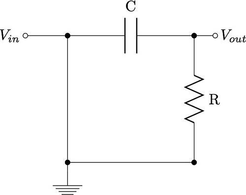
The frequency response of an ideal LPF is characterized by a brick-wall transition at $$f_c$$, but real-world filters exhibit a gradual roll-off. The transfer function $$H(f)$$ of a first-order passive RC LPF is derived from Kirchhoff’s laws:
where $$R$$ is resistance, $$C$$ is capacitance, and $$j$$ is the imaginary unit. The magnitude response in decibels (dB) is:
The cutoff frequency $$f_c$$ is defined as the point where the power drops to half (-3 dB) of the passband value:
Practical Applications
- Anti-aliasing: LPFs are critical in analog-to-digital converters (ADCs) to enforce the Nyquist criterion by eliminating frequencies above half the sampling rate.
- Noise suppression: High-frequency noise from power supplies or RF interference is attenuated in sensor signal conditioning.
- Audio processing: LPFs shape the frequency response in speakers and audio amplifiers to limit ultrasonic content.
Real-World Tradeoffs
Practical LPFs deviate from ideal behavior due to:
- Roll-off rate: Determined by filter order (e.g., 20 dB/decade for first-order). Higher-order filters (Butterworth, Chebyshev) offer steeper transitions but introduce phase distortion.
- Passband ripple: Tolerable amplitude variations in the passband, often minimized in Bessel or elliptic filters.
- Group delay: Nonlinear phase response in higher-order filters can distort transient signals.
Design Considerations
Selecting an LPF topology depends on:
- Active vs. passive: Active filters (using op-amps) provide gain and sharper roll-off but require power supplies.
- Component tolerance: RC networks are simple but sensitive to component variations; switched-capacitor filters offer precision at the cost of clock noise.
Frequency Response Characteristics
The frequency response of a low-pass filter (LPF) defines how the filter attenuates or passes signals as a function of frequency. For an ideal LPF, the gain is unity (0 dB) in the passband and zero in the stopband, with an instantaneous transition at the cutoff frequency. However, real filters exhibit gradual roll-off and non-ideal behavior, which can be rigorously analyzed using transfer functions and Bode plots.
Transfer Function of a First-Order RC Low-Pass Filter
The simplest LPF is the first-order RC filter, characterized by a single pole in its transfer function. The voltage across the capacitor (Vout) relative to the input voltage (Vin) is given by:
where R is the resistance, C the capacitance, and ω the angular frequency (ω = 2πf). The magnitude and phase response are derived as:
The cutoff frequency (fc), where the output power is halved (−3 dB point), occurs when ωRC = 1:
Second-Order and Higher-Order Filter Responses
Higher-order filters provide steeper roll-off rates, critical for applications requiring sharp transition bands. A second-order LPF, such as a Butterworth filter, has a transfer function:
where Q (quality factor) determines the damping and peaking near the cutoff frequency. For a Butterworth filter (maximally flat passband), Q = 0.707, yielding a roll-off of −40 dB/decade.
Key Frequency Response Metrics
- Passband Ripple: Variations in gain within the passband (e.g., ±0.5 dB for Chebyshev filters).
- Stopband Attenuation: Minimum attenuation in the stopband (e.g., −60 dB for anti-aliasing filters).
- Transition Band Slope: Roll-off rate (e.g., −20n dB/decade for an n-th order filter).
Bode Plot Analysis
A Bode plot visualizes the magnitude (in dB) and phase (in degrees) responses. For a first-order LPF:
- Magnitude: Flat at 0 dB until fc, then rolls off at −20 dB/decade.
- Phase: Shifts from 0° to −90°, with −45° at fc.
For a second-order Butterworth filter, the phase shift extends to −180°, and the magnitude roll-off doubles to −40 dB/decade.
Practical Implications
In RF and audio systems, LPFs suppress high-frequency noise and harmonics. For example, a 5th-order LPF in a DAC reconstruction filter ensures negligible aliasing artifacts. The choice of filter type (Butterworth, Chebyshev, Bessel) trades off roll-off steepness, phase linearity, and passband ripple.
Cutoff Frequency and Roll-off
Definition of Cutoff Frequency
The cutoff frequency (fc) of a low-pass filter is the frequency at which the output signal power is reduced to half (-3 dB) of its maximum passband value. This corresponds to the point where the voltage gain drops to
Derivation of the -3 dB Point
The -3 dB reference arises from the logarithmic decibel scale, where power ratio is expressed as:
At fc, the output power is halved, leading to:
Roll-off Rate
The roll-off rate describes how rapidly the filter attenuates signals beyond fc. For an n-th order filter, the roll-off is:
For example, a first-order filter (n = 1) attenuates at 20 dB/decade, while a second-order Butterworth filter achieves 40 dB/decade.
Phase Response and Group Delay
Near fc, the phase shift introduced by a first-order filter is -45°. The group delay, defined as the negative derivative of phase with respect to angular frequency (τ_g = -d\phi/dω), is critical for preserving signal integrity in time-domain applications. For an RC filter:
Practical Implications
- Aliasing Prevention: In analog-to-digital conversion, the filter’s roll-off must suppress frequencies above the Nyquist rate.
- Audio Systems: Loudspeaker crossovers use steep roll-offs (e.g., 24 dB/octave Linkwitz-Riley filters) to isolate frequency bands.
- Communication Systems: Raised-cosine filters optimize roll-off to minimize inter-symbol interference (ISI).
Higher-Order Filters and Roll-off Enhancement
Butterworth, Chebyshev, and Bessel filters trade off roll-off steepness for passband ripple or phase linearity. For instance, an 8th-order Chebyshev filter can achieve >100 dB/decade roll-off but introduces passband ripple:
where Tn is the Chebyshev polynomial of order n, and ϵ controls ripple magnitude.
2. Passive Low Pass Filters
2.1 Passive Low Pass Filters
Passive low pass filters (LPFs) are fundamental building blocks in signal processing, constructed using only passive components—resistors, capacitors, and inductors—without amplification. Their operation relies on frequency-dependent impedance to attenuate high-frequency signals while allowing low-frequency components to pass.
First-Order RC Low Pass Filter
The simplest passive LPF is the first-order RC filter, consisting of a resistor R and capacitor C in series. The transfer function H(f) describes the output-to-input voltage ratio as a function of frequency:
The magnitude response, calculated as |H(f)|, reveals the filter's attenuation characteristics:
The cutoff frequency fc, where the output power drops to half (-3 dB) of the input, is derived by setting |H(f)| = 1/√2:
First-Order RL Low Pass Filter
An alternative implementation replaces the capacitor with an inductor L. The transfer function and cutoff frequency for this RL configuration are:
While RL filters are less common due to inductor non-idealities (e.g., parasitic resistance and size), they remain relevant in high-current applications where capacitors are impractical.
Second-Order Passive LC Filters
Higher-order filters improve roll-off steepness. A second-order LPF combines L and C to form an LC tank circuit. The transfer function for this RLC configuration is:
The cutoff frequency and quality factor Q are critical design parameters:
A high Q (>0.707) introduces peaking near fc, while Q = 0.707 yields a Butterworth response with maximally flat passband.
Practical Considerations
- Component Tolerances: Passive filters are sensitive to R, L, and C variations, requiring precision components for critical applications.
- Impedance Matching: Source and load impedances affect the cutoff frequency and attenuation. Buffering may be necessary to isolate the filter.
- Parasitics: Stray capacitance and inductor resistance degrade high-frequency performance, limiting usable bandwidth.
Applications
Passive LPFs are ubiquitous in:
- Audio systems (e.g., crossover networks)
- Radio frequency (RF) signal conditioning
- Power supply ripple reduction
- Anti-aliasing in analog-to-digital converters
2.2 Active Low Pass Filters
Active low pass filters incorporate operational amplifiers (op-amps) to provide gain and improve performance compared to passive RC filters. The op-amp's high input impedance prevents loading effects, while its low output impedance ensures signal integrity when driving subsequent stages. These filters are widely used in audio processing, anti-aliasing in ADCs, and noise reduction in communication systems.
First-Order Active Low Pass Filter
The simplest active low pass filter is a first-order design, consisting of an RC network followed by a non-inverting op-amp configuration. The transfer function H(s) of this circuit is derived as:
Here, Rf and Ri set the DC gain A0, while R and C determine the cutoff frequency fc:
The Bode plot of this filter shows a -20 dB/decade roll-off above fc, characteristic of first-order systems. The op-amp's bandwidth must exceed fc to avoid signal degradation.
Second-Order Active Low Pass Filter
For steeper roll-off, second-order active filters are employed. The Sallen-Key topology is a common implementation, using two RC pairs and an op-amp configured as a voltage follower or amplifier. Its transfer function is:
Where A0 is the DC gain set by the feedback network. The quality factor Q and cutoff frequency are:
Proper selection of component values ensures a Butterworth, Chebyshev, or Bessel response, depending on the application's need for flat passband, sharp transition, or phase linearity.
Higher-Order Filters
Cascading multiple second-order stages achieves higher-order filtering. For instance, a fourth-order filter can be constructed by cascading two second-order Sallen-Key circuits. Each stage's Q and fc must be carefully tuned to avoid peaking and maintain stability. The overall transfer function becomes the product of individual stage responses:
Active filters with orders beyond four are practical but require precision components to mitigate cumulative errors from op-amp non-idealities like finite gain-bandwidth product and slew rate.
Design Considerations
Key parameters in active filter design include:
- Op-amp selection: Choose devices with sufficient bandwidth, low noise, and low distortion (e.g., FET-input op-amps for high-impedance nodes).
- Component tolerance: Use 1% resistors and NPO/COG capacitors to minimize deviation from the desired response.
- Power supply rejection: Decouple supply rails to prevent noise coupling into the filter's passband.
Modern active filters often integrate programmable components (e.g., digital potentiometers or switched capacitors) for adjustable cutoff frequencies in adaptive systems.
First-Order vs. Second-Order Filters
Transfer Function and Frequency Response
The fundamental distinction between first-order and second-order low-pass filters lies in their transfer functions and roll-off rates. A first-order filter has a transfer function given by:
where s is the complex frequency variable and ωc is the cutoff frequency. The magnitude response decays at −20 dB/decade beyond the cutoff frequency.
In contrast, a second-order filter has a transfer function:
where Q is the quality factor, influencing the filter's resonance and damping. The roll-off rate is −40 dB/decade, providing steeper attenuation.
Pole-Zero Analysis
First-order filters have a single pole at s = −ωc, resulting in a smooth, monotonic frequency response. Second-order filters, however, exhibit complex conjugate poles when Q > 0.5, leading to peaking near the cutoff frequency. The pole locations are determined by:
Higher Q values increase resonance, while lower values (Q < 0.5) result in overdamped behavior with two real poles.
Phase Response and Group Delay
First-order filters introduce a phase shift of −90° at high frequencies, with a gradual transition. Second-order filters exhibit a phase shift of −180°, but the transition is steeper and influenced by Q. The group delay, defined as the negative derivative of phase with respect to frequency, is more pronounced in second-order filters, particularly near resonance.
Practical Implementation
First-order filters are typically implemented using a single resistor-capacitor (RC) network, making them simple and cost-effective. Second-order filters require additional components, such as inductors or active elements (e.g., op-amps), to achieve the desired response. Common topologies include:
- Sallen-Key (active, voltage-controlled)
- Multiple Feedback (MFB) (active, inverting)
- RLC (passive, resonant)
Applications and Trade-offs
First-order filters are suitable for applications requiring minimal component count and moderate roll-off, such as basic signal conditioning. Second-order filters are preferred in scenarios demanding sharper attenuation, such as anti-aliasing in ADCs or noise suppression in RF circuits. However, they introduce trade-offs in terms of complexity, component tolerance sensitivity, and potential stability issues in active implementations.
Design Considerations
When selecting between first-order and second-order filters, key considerations include:
- Roll-off requirement: Second-order filters provide superior stopband rejection.
- Phase linearity: First-order filters exhibit more predictable phase behavior.
- Component sensitivity: Second-order active filters are sensitive to op-amp bandwidth and resistor/capacitor tolerances.
3. Component Selection (Resistors, Capacitors, Op-Amps)
3.1 Component Selection (Resistors, Capacitors, Op-Amps)
The performance of a low-pass filter (LPF) is critically dependent on the choice of passive and active components. Key parameters such as cutoff frequency, phase response, and signal integrity are directly influenced by resistor and capacitor tolerances, op-amp bandwidth, and noise characteristics.
Resistor Selection
Resistors in an LPF define the time constant τ = RC, which determines the cutoff frequency fc. For a first-order passive RC filter:
Key considerations for resistor selection include:
- Tolerance: Standard resistors have ±5%, ±1%, or ±0.1% tolerances. Tight tolerance (±0.1%) minimizes deviation in fc.
- Temperature Coefficient (TCR): Low TCR (<10 ppm/°C) reduces drift with temperature.
- Noise: Metal-film resistors exhibit lower thermal noise than carbon composition.
For high-frequency applications, parasitic inductance (Lpar) becomes significant. Thin-film SMD resistors (e.g., 0603 or 0402 packages) minimize parasitic effects.
Capacitor Selection
Capacitors introduce frequency-dependent impedance ZC = 1/(jωC). The choice of dielectric material impacts stability and losses:
- Ceramic (C0G/NP0): Low ESR, minimal dielectric absorption, stable across temperature.
- Polypropylene/Polyester: Low leakage, suitable for precision analog filters.
- Electrolytic/Tantalum: Avoid in signal paths due to high ESR and polarity constraints.
Voltage derating (operating at ≤80% of rated voltage) improves longevity. For second-order filters, capacitor matching (±1% or better) ensures balanced pole placement.
Operational Amplifier Selection
Active LPFs rely on op-amps to provide gain and buffer stages. Critical op-amp parameters include:
- Gain-Bandwidth Product (GBW): Must exceed the filter's operating frequency (typically 5–10× fc).
- Slew Rate (SR): Limits maximum undistorted output swing at high frequencies (SR > 2πfVpeak).
- Input Noise Density: Voltage noise (nV/√Hz) and current noise (pA/√Hz) degrade SNR.
For example, a Butterworth LPF with fc = 10 kHz and Vpeak = 5 V requires:
Precision op-amps like the OPA1611 (GBW = 40 MHz, SR = 20 V/μs) are suitable for high-fidelity applications, whereas low-power designs may use the LTC6258 (GBW = 12.5 MHz, SR = 5 V/μs).
Practical Design Example
Consider a Sallen-Key second-order LPF with fc = 1 kHz and Q = 0.707 (Butterworth response). Component values are derived as:
Using 1% tolerance metal-film resistors (10 kΩ) and C0G ceramic capacitors (16 nF) ensures fc accuracy within ±2%. An op-amp with GBW > 1 MHz (e.g., TL072) suffices for this application.
This section provides a rigorous, application-focused guide to component selection for low-pass filters, balancing theoretical foundations with practical design constraints. The mathematical derivations and real-world examples cater to advanced readers while maintaining readability through structured explanations.Transfer Function and Bode Plots
Transfer Function of a Low-Pass Filter
The transfer function H(s) of a low-pass filter characterizes its frequency response in the Laplace domain. For a first-order RC low-pass filter, the transfer function is derived from the voltage divider principle:
where ZC = 1/(sC) is the impedance of the capacitor and ZR = R is the resistor's impedance. Substituting these yields:
The pole frequency ωc = 1/(RC) defines the cutoff frequency. Rewriting H(s) in standard form:
Frequency Response and Bode Plots
To analyze the filter's behavior in the frequency domain, substitute s = jω:
The magnitude response |H(jω)| and phase response ∠H(jω) are:
A Bode plot visualizes these responses using logarithmic scales. The magnitude plot (in dB) has two asymptotic regions:
- For ω ≪ ωc: |H(jω)| ≈ 1 (0 dB flat response)
- For ω ≫ ωc: |H(jω)| ≈ ωc/ω (-20 dB/decade rolloff)
The phase plot transitions from 0° to -90°, with -45° at ω = ωc.
Second-Order Low-Pass Filters
For a second-order RLC filter, the transfer function includes a damping factor ζ and resonant frequency ω0:
The Bode plot shows a steeper -40 dB/decade rolloff above ω0, with peaking near ω0 if ζ < 0.707.
Practical Applications
Bode plots are indispensable for:
- Predicting signal attenuation in audio processing
- Analyzing stability in feedback control systems
- Designing anti-aliasing filters for ADCs
3.3 Practical Design Considerations
When designing a low pass filter (LPF), theoretical transfer functions must be reconciled with real-world component behavior. Non-idealities such as parasitic capacitance, inductor series resistance, and op-amp bandwidth limitations significantly alter performance.
Component Tolerances and Temperature Effects
Passive components exhibit manufacturing tolerances (typically ±5% for resistors, ±10% for capacitors). For a second-order active LPF with cutoff frequency fc:
A 10% tolerance in both R and C can shift fc by ±20%. Temperature coefficients further exacerbate this:
- Resistors: 100-200 ppm/°C for metal film
- Capacitors: X7R ceramics (±15% over -55°C to +125°C)
Op-Amp Limitations
The finite gain-bandwidth product (GBW) of operational amplifiers imposes practical constraints. For an active LPF using a non-ideal op-amp:
where AOL is the open-loop gain and β(s) the feedback factor. To maintain stability:
For a Butterworth filter (Q=0.707) with fc=10 kHz, GBW must exceed 50 MHz.
PCB Layout Considerations
Parasitic capacitance between traces (Cp ≈ 0.2-1 pF/cm) and inductance of component leads (Lp ≈ 1-10 nH) create unintended poles. Mitigation strategies include:
- Ground planes to minimize loop inductance
- Surface-mount components to reduce lead parasitics
- Star routing for high-impedance nodes
Power Supply Rejection
Active filters require clean power rails. Power supply rejection ratio (PSRR) of modern op-amps degrades above 10 kHz. A bypass capacitor network is essential:
Typical values: 10 µF tantalum (bulk) + 100 nF X7R (high-frequency).
Noise Analysis
Thermal noise from resistors and voltage noise from op-amps contribute to the output noise spectral density:
For a 1 kΩ resistor at 25°C, 4kTR = 16 nV/√Hz. Low-noise design requires:
- JFET-input op-amps for high-Z circuits
- Parallel resistors to reduce thermal noise
- Bandwidth limiting post-filtering
4. Signal Processing and Noise Reduction
4.1 Signal Processing and Noise Reduction
Low-pass filters (LPFs) are fundamental in signal processing for attenuating high-frequency noise while preserving the integrity of low-frequency signals. Their operation is rooted in the frequency-dependent impedance characteristics of reactive components—capacitors and inductors. The simplest first-order RC LPF has a transfer function H(f) given by:
where fc is the cutoff frequency, defined as:
For noise reduction, the filter's roll-off rate is critical. A first-order LPF provides -20 dB/decade attenuation beyond fc, while higher-order filters (e.g., Butterworth, Chebyshev) achieve steeper roll-offs. The Butterworth filter, for instance, maximizes flatness in the passband with a transfer function magnitude:
where n is the filter order. Practical implementations often use active filters (e.g., Sallen-Key topology) to avoid loading effects and improve Q-factor.
Noise Reduction Mechanisms
LPFs suppress noise by exploiting the spectral separation between signal and noise. Key considerations include:
- White Noise: Uniformly distributed across frequencies. An LPF attenuates noise power proportionally to bandwidth reduction.
- 1/f Noise: Dominant at low frequencies; requires careful cutoff selection to avoid signal degradation.
- Aliasing: In ADC systems, LPFs (anti-aliasing filters) must attenuate frequencies above the Nyquist rate.
Design Trade-offs
Filter design involves balancing:
- Cutoff Frequency: Lower fc improves noise rejection but may distort transient signals.
- Phase Linearity: Bessel filters preserve phase at the cost of slower roll-off.
- Group Delay: Critical in communication systems to avoid intersymbol interference.
Practical Applications
LPFs are ubiquitous in:
- Audio Systems: Removing ultrasonic noise before amplification.
- Sensor Interfaces: Mitigating high-frequency environmental interference.
- Power Supplies: Smoothing rectified AC ripple.
Low Pass Filters in Audio Systems and Communication
:Frequency Response in Audio Applications
In audio systems, low pass filters (LPFs) are critical for bandwidth limiting and anti-aliasing. The human auditory range spans 20 Hz to 20 kHz, but practical systems often restrict bandwidth to minimize noise and distortion. A first-order RC LPF with cutoff frequency fc is defined by:
For high-fidelity audio, higher-order filters (Butterworth, Chebyshev) are preferred due to their steeper roll-off. A second-order Butterworth LPF, for instance, attenuates signals at −40 dB/decade beyond fc, given by:
Phase Linearity and Group Delay
LPFs introduce phase shifts, which can distort transient signals like percussion. A Bessel filter preserves phase linearity, sacrificing roll-off steepness. The group delay τg, defined as the negative derivative of phase with respect to angular frequency, is nearly constant for Bessel filters:
Communication Systems: Channel Noise and ISI
In RF and wired communication, LPFs mitigate inter-symbol interference (ISI) by band-limiting transmitted signals. The raised-cosine filter, a hybrid LPF, minimizes ISI while optimizing spectral efficiency. Its transfer function combines an LPF with a tunable roll-off factor α:
Practical Implementation: Active vs. Passive Filters
Active LPFs using op-amps (e.g., Sallen-Key topology) avoid loading effects and provide gain. For instance, a Sallen-Key second-order LPF with unity gain has:
Passive LC filters, however, are favored in high-power RF applications due to their linearity and lack of active noise sources.
Case Study: LPF in Digital Audio Workstations (DAWs)
Modern DAWs use FIR-based LPFs with linear phase for mastering. An FIR filter of order N applies convolution:
where h[k] are coefficients designed via windowing or Parks-McClellan optimization.
4.3 Power Supply Filtering
Power supply noise, often manifesting as high-frequency ripple or transient disturbances, degrades the performance of sensitive analog and digital circuits. A low-pass filter (LPF) is critical in attenuating this noise while preserving the DC component of the supply voltage. The design parameters—cutoff frequency, roll-off slope, and component selection—directly impact the filter's efficacy.
Transfer Function and Impedance Considerations
The LPF for power supplies typically employs an RC or LC topology. The transfer function for an RC filter is:
where R represents the equivalent series resistance (ESR) of the capacitor, and C is the filtering capacitance. For an LC filter, the transfer function becomes:
The LC configuration offers a steeper roll-off (−40 dB/decade) compared to the RC filter (−20 dB/decade), but requires careful damping to avoid resonance peaks. The quality factor (Q) must be minimized to prevent ringing:
Component Selection and Practical Trade-offs
Key considerations include:
- Capacitor ESR: Low ESR (e.g., ceramic or polymer capacitors) reduces voltage drop at high frequencies but may necessitate additional damping.
- Inductor Saturation Current: Must exceed the maximum load current to avoid nonlinearity.
- Parasitics: Stray inductance in capacitors and parasitic capacitance in inductors can shift the cutoff frequency.
A multi-stage approach is common in high-performance systems. For example, a bulk electrolytic capacitor (10–100 µF) handles low-frequency ripple, while a ceramic capacitor (0.1–1 µF) suppresses high-frequency noise.
Real-World Applications
In switch-mode power supplies (SMPS), a second-stage LPF with a cutoff frequency below the switching frequency (e.g., 50 kHz for a 200 kHz SMPS) is essential. For precision analog circuits (e.g., ADCs or oscillators), a ferrite bead in series with a capacitor forms a broadband filter, attenuating both conducted and radiated interference.
Modern integrated voltage regulators (e.g., LDOs) often embed active filtering, but discrete LPFs remain necessary for high-current or ultra-low-noise scenarios. SPICE simulations are recommended to validate the design under transient and load-variation conditions.
5. Key Textbooks and Papers
5.1 Key Textbooks and Papers
- Electronic filters : theory, numerical recipes, and design practice ... — Stanford Libraries' official online search tool for books, media, journals, databases, ... Electronic filters : theory, numerical recipes, and design practice based on the RM software ... 5.5 Possible Transfer Functions; 5.5.1 Low-Pass Filters; 5.5.1.1 Selective Polynomial Filters; 5.5.1.2 Polynomial Linear Phase Monotonic Pass-Band-Amplitude ...
- PDF Butterworth Low-pass Filter Design — 2.1 THEORY OF MICROWAVE FILTERS 5 2.1.1 Ideal Microwave filters 5 2.1.2 Microwave Filter Design 6 2.2 Low-pass filter 7 2.3 Butterworth (maximally flat) low-pass filter 8 2.4 Butterworth Low-Pass Filter Design 9 2.5 Transformation from lumped elements to distributed elements 11 CHAPTER 3 12 3.1 Design and Simulation Procedure 12 3.2 Genesys 13
- PDF Chapter 5 Design of IIR Filters - Newcastle University — Ideal low-pass filter Butterworth filter Chebyshev filter Elliptic filter Frequency ω H(ω) ωo Pass-band ripple = 0.5 dB Filter order n =3 ωo = 0.5 Figure 5.1: Typical frequency responses of various analogue low-pass filters. 5.4 The Bilinear z-transform
- (PDF) Active Low-Pass Filter Design - Academia.edu — Fifth-Order Low-Pass Filter Topology Cascading Two Sallen-Key Stages and an RC 22 Active Low-Pass Filter Design VO SLOA049B B.1.2 Sixth-Order Low-Pass Bessel Filter ǒǒ Ǔǒ ǒ Ǔǒ ǒ Referring to Table 2 for a sixth-order Bessel filter, we can write the required circuit transfer function as: H LP(f) + - f 1.6060fc Ǔ) 2 1.2202 jf fc )1 ...
- PDF Chapter 5 : FILTERS — The theory underlying design of electronic filters is formidable. We confine our discussion of filters to the extent necessary to implement the filters used in TRC-10, in this chapter. 5.1. Motivation Any electronic filter can be visualized as a block between a source (input) and a load (output). This is depicted in Figure 5.1.
- What Is a Low Pass Filter? Understanding Electronic Filter — A negative dB value implies a reduction in output signal strength. Therefore, a negative dB value indicates attenuation, and a high-frequency signal has been rejected by the low-pass filter. Low Pass Filter Key Characteristics. The low-pass filter is a reliable electronic circuit that performs the role of attenuating high-frequency signals.
- PDF Importance of High Order High Pass and Low Pass Filters - ResearchGate — World Appl. Sci. J., 34 (9): 1261-1268, 2016 1265 A high pass filter is design to pass all frequencies Figure 4.6 is the PHPF with inductance that has been design, they have a lot of merits.
- PDF Active Filter Design Techniques - School of Engineering & Applied Science — The Bessel low-pass filters have a linear phase response (Figure 16 - 7) over a wide fre-quency range, which results in a constant group delay (Figure 16- 8) in that frequency range. Bessel low-pass filters, therefore, provide an optimum square-wave transmission behavior. However, the passband gain of a Bessel low-pass filter is not as flat ...
- Active Low-Pass Filter Design (Rev. D) - Texas Instruments — Active Low-Pass Filter Design Jim Karki AAP Precision Analog ABSTRACT This report focuses on active low-pass filter design using operational amplifiers. Low-pass filters are commonly used to implement anti-aliasing filters in data acquisition systems. Design of second-order filters is the main topic of consideration.
- 5.1.9. Low Pass Filter — Digital Signal Processing — This filter is called a first order filter as the radial frequency occurs linearly in the formula (exponent 1). In an exercise you are asked to plot the phase change of the filter. In speaker design one strives for as little phase change as possible. The low pass filter detailed here is the simplest of them all. We can make more complex filters.
5.2 Online Resources and Tutorials
- 5.2.9. Low Pass Filter — Signal Processing 1.1 documentation — Sallen Key opamp filter; 5.2.14.9. Audio Equalizer; 5.3. Sampling. 5.3.1. The Sampling Theorem; 5.3.2. Interpolation. ... Analog Electronics » 5.2.9. Low Pass Filter; View page source; Next Previous. ... In other words we need a low pass filter. An ideal low pass filter is just an ideal, you can't make it.
- 5.2.14. Excercises — Signal Processing 1.1 documentation — Analog Electronics » 5.2.14. Excercises ... 5.2.14.8. Sallen Key opamp filter ... Can you make a first order low-pass filter by a clever choice of the resistor and capacitor values starting from the generic Sallen-Key filter? Show that replacing a resistor with a capacitor and vice versa will change the high-pass filter into a low-pass filter.
- PDF Part 2 Filters - University of Oxford — Figure 22: Various passive low-pass filters. The simplest passive filter can be created using a resistor and capacitor. An example of this type of circuit designed to be a low-pass filter is shown in Figure (22 (a)). The response of this type of filter, is which can be re-written as
- PDF Active Low-Pass Filter Design (Rev. B) - TI E2E support forums — overshoot and ringing than a Butterworth filter. 3 Second-Order Low-Pass Filter - Standard Form The transfer function HLP of a second-order low-pass filter can be express as a function of frequency (f) as shown in Equation 1. We shall use this as our standard form. HLP(f) K f FSF fc 2 1 Q jf FSF fc 1 Equation 1. Second-Order Low-Pass Filter ...
- PDF Chapter 5 Design of IIR Filters - Newcastle University — The design of analogue filters other than low-pass is usually achieved by designing a low-pass filter of the desired class e.g. Butterworth, Chebyshev, or Elliptic, and then transforming the resulting filter to get the desired frequency response e.g. high-pass, band-pass, or band-stop.
- Passive Band Pass Filter - Passive RC Filter Tutorial — The Passive Band Pass Filter can be used to isolate or filter out certain frequencies that lie within a particular band or range of frequencies. The cut-off frequency or ƒc point in a simple RC passive filter can be accurately controlled using just a single resistor in series with a non-polarized capacitor, and depending upon which way around they are connected, we have seen that either a Low ...
- Active Low-Pass Filter Design (Rev. D) - Texas Instruments — Active Low-Pass Filter Design Jim Karki AAP Precision Analog ABSTRACT This report focuses on active low-pass filter design using operational amplifiers. Low-pass filters are commonly used to implement anti-aliasing filters in data acquisition systems. Design of second-order filters is the main topic of consideration.
- PHYS 3330 - Filters — Website of Electronics Lab - PHYS 3330. Toggle navigation PHYS 3330 - Electronics Lab. Home; Lab Guides; ... Low-pass filter - a filter that passes low frequency signals and attenuates (reduces the amplitude of) signals with frequencies higher than the cutoff frequency. Also known as an integrator. ... check out this resource. 5 Prelab 5.1 ...
- PDF Chapter 5 : FILTERS — The theory underlying design of electronic filters is formidable. We confine our discussion of filters to the extent necessary to implement the filters used in TRC-10, in this chapter. 5.1. Motivation Any electronic filter can be visualized as a block between a source (input) and a load (output). This is depicted in Figure 5.1.
- PDF LC Filter Design (Rev. A) - Texas Instruments — LC Filter Design All trademarks are the property of their respective owners. Application Report ... 5 2.1 AD (Traditional) Modulation ... Two considerations when selecting components for the second-order low-pass filter is the cut-
5.3 Advanced Topics for Further Study
- Solved Section 5.3: Low- and High-Pass Filters 5.11 a. - Chegg — Section 5.3: Low- and High-Pass Filters 5.11 a. Determine the frequency response Vorut G)/V.. (w) for the circuit of Figure P5.11. Assume L = 0.5 H and R = 200 k22. b. Plot the magnitude and phase of the circuit for frequencies between 10 and 10' rad/s on graph paper, with a linear scale for frequency. c. Repeat part b. using semilog paper.
- PDF Lab 3: Low Pass and High Pass Filters - The University of Texas at Dallas — • Passive Low-Pass Filter, • Active Low-Pass Filter, • Passive High-Pass Filter, and • Active High-Pass Filter. For each of the configurations you will 1. Design the filter for a specified cut-off frequency, 2. Model the filter in MatLab, 3. 2Simulate the design with PSpice, and 4. Test the design in the Lab.
- Low-Pass and High-Pass Filters | UCSC Physics Demonstration Room — An important note is that this equation holds for both high-pass and low-pass RC filters with the same resistor and capacitor. For a low-pass filter, increasing past the cutoff frequency will cause the output amplitude to drop. As for the high-pass filter, decreasing the frequency below the cutoff will cause a similar decrease in output voltage.
- Electronic filters : theory, numerical recipes, and design practice ... — Further, it discusses new procedures to improve the selectivity of all polynomial filters by introducing transmission zeros, such as filters with multiple transmission zeros on the omega axis, as well as phase correction of selective filters for both low-pass and band-pass filters. Other topics explored include linear phase all-pass (exhibiting ...
- PDF Active Low-Pass Filter Design (Rev. D) - Texas Instruments — Active Low-Pass Filter Design Jim Karki AAP Precision Analog ABSTRACT This report focuses on active low-pass filter design using operational amplifiers. Low-pass filters are commonly used to implement anti-aliasing filters in data acquisition systems. Design of second-order filters is the main topic of consideration.
- 5.3. Filters — Digital Signal Processing - Universiteit van Amsterdam — The characterization of analog filters is most often done in the \(s\)-domain. In this chapter we will look at several filter prototypes characterized in the \(s\)-domain. Starting from a prototype for a low-pass filter we can transform the filter to act as a high-pass filter, or as a band-pass or a band-reject (notch) filter.
- PDF Chapter 5 : FILTERS — The theory underlying design of electronic filters is formidable. We confine our discussion of filters to the extent necessary to implement the filters used in TRC-10, in this chapter. 5.1. Motivation Any electronic filter can be visualized as a block between a source (input) and a load (output). This is depicted in Figure 5.1.
- PDF ECE-205 Lab 10 Lowpass, Highpass, and Bandpass Filters — subsystems. The first subsystem is the lowpass filer, the second subsystem is the highpass filter, and the last subsystem is an all pass filter which just adjusts the gain of the system. As with most of the circuits in this class, this design has not been optimized and is very inefficient, but should be fairly easy to build. All of the resistors
- Ladder Filters: Butterworth & Chebyshev - Lecture Notes - studylib.net — Equal Ripple, or Chebyshev Low Pass Filter The values of the inductors and capacitors in this type of filter are somehow chosen so that P (5.3) LC f i 1 Cn2 f fc P argument In this expression: = ripple size, f Cn f Chebyshev polynomial of order n (see plots in Fig. n 5.3b), Chebyshev filters might be more susceptible to variations in component ...
- PDF EECE 301 Signals & Systems Prof. Mark Fowler - Binghamton University — 5.3 Ideal Filters Often we have a scenario where we have a "good" signal, x g (t), corrupted by a "bad" signal, x b (t), and we want to use an LTI system to remove (or filter out) the bad signal, leaving only the good signal. How do we do this?