Magnetism
1. Definition and Basic Properties
1.1 Definition and Basic Properties
Fundamental Nature of Magnetism
Magnetism arises from the motion of electric charges, a phenomenon fundamentally rooted in relativistic quantum electrodynamics. At the atomic level, two primary contributions generate magnetic moments: orbital angular momentum of electrons around nuclei and intrinsic spin, a purely quantum mechanical property. The total magnetic moment μ of an atom can be expressed as:
where μB is the Bohr magneton (9.27 × 10⁻²⁴ J/T), L and S are orbital and spin angular momentum operators, and g ≈ 2 is the electron g-factor. In ferromagnetic materials like iron, unpaired electron spins align collectively, producing macroscopic magnetization.
Magnetic Field Quantification
The magnetic field B (flux density) and auxiliary field H (field intensity) relate through material properties:
where M is magnetization (dipole moment per unit volume), μ0 is vacuum permeability (4π × 10-7 N/A2), and μr is relative permeability. For anisotropic materials, μr becomes a tensor. The distinction between B and H is critical in nonlinear media, where hysteresis effects dominate.
Classification of Magnetic Materials
Materials respond to external fields through their magnetic susceptibility χm:
- Diamagnets (χm ≈ -10-5): Induce weak opposing fields via Lenz's law (e.g., bismuth, superconductors).
- Paramagnets (χm ≈ 10-3): Partially align moments with thermal disruption (e.g., aluminum, oxygen).
- Ferromagnets (χm ≫ 1): Exhibit spontaneous alignment below Curie temperature (e.g., iron, cobalt).
- Antiferromagnets: Neighboring spins antiparallel (e.g., MnO, chromium).
- Ferrimagnets: Unequal antiparallel moments (e.g., magnetite, ferrites).
Maxwell's Equations for Magnetostatics
In static conditions, magnetic fields obey:
These imply B forms solenoidal fields, while H circulates around current densities J. The vector potential A, where B = ∇ × A, simplifies calculations in boundary-value problems.
Practical Implications
Magnetic properties dictate device performance in:
- Power systems: Transformer cores require high-μ silicon steel to minimize hysteresis losses.
- Data storage: Hard drives exploit ferromagnetic domain switching with coercivities tuned for stability.
- Medical imaging: MRI scanners use superconducting magnets producing >1.5 T fields for nuclear spin alignment.
The diagram illustrates magnetic domains in a ferromagnet. Arrows represent local magnetization vectors, which align under external fields, causing bulk magnetization. Domain walls are regions where spin orientations transition, typically 10-100 nm wide in transition metals.
1.2 Magnetic Fields and Flux
Definition of Magnetic Field
The magnetic field B is a vector field that describes the magnetic influence on moving electric charges, electric currents, and magnetic materials. It is defined operationally by the Lorentz force law:
where F is the force experienced by a charge q moving with velocity v. The SI unit of magnetic field is the tesla (T), equivalent to N·A⁻¹·m⁻¹.
Magnetic Field Lines
Magnetic fields are visualized using field lines, which are continuous curves tangent to the field vector at every point. Key properties:
- Lines emerge from north poles and terminate at south poles.
- Line density represents field strength.
- Lines never intersect (uniqueness theorem for divergence-free fields).
Magnetic Flux
Magnetic flux Φ through a surface S is defined as the surface integral:
where dA is the differential area vector. For a uniform field perpendicular to a flat area A, this simplifies to:
Gauss's Law for Magnetism
One of Maxwell's equations states:
In integral form, this becomes:
This implies there are no magnetic monopoles - all field lines form closed loops.
Practical Applications
Magnetic flux concepts are fundamental to:
- Transformer design (flux linkage between windings)
- Electric generators (time-varying flux induces EMF)
- Magnetic shielding (divergence-free nature of B fields)
- MRI machines (precise flux measurements for imaging)
Advanced Considerations
For time-dependent systems, Faraday's law relates changing flux to induced EMF:
In materials, the magnetic field H and flux density B are related by:
where M is the magnetization and μ₀ is the permeability of free space (4π×10⁻⁷ N·A⁻²).
1.3 Types of Magnetic Materials
Magnetic materials are classified based on their response to an external magnetic field, characterized by their magnetic susceptibility (χ) and permeability (μ). The primary categories include diamagnetic, paramagnetic, ferromagnetic, antiferromagnetic, and ferrimagnetic materials, each exhibiting distinct microscopic and macroscopic behaviors.
Diamagnetic Materials
Diamagnetic materials possess no intrinsic magnetic moment. When subjected to an external magnetic field, electron orbits adjust to generate a weak opposing magnetization, resulting in negative susceptibility (χ < 0). The magnetic permeability is slightly less than unity (μ < μ0). This effect, governed by Lenz's law, is present in all materials but is often overshadowed by stronger magnetic responses. Examples include bismuth, copper, and water. Diamagnetism finds applications in magnetic levitation, such as superconducting quantum interference devices (SQUIDs).
Paramagnetic Materials
Paramagnetic materials contain unpaired electrons that align with an external field, producing a weak positive susceptibility (χ > 0). Unlike ferromagnets, thermal agitation prevents spontaneous magnetization, and the effect is temperature-dependent, as described by Curie's law:
where C is the Curie constant and T is temperature. Examples include aluminum and oxygen. Paramagnetism is exploited in magnetic resonance imaging (MRI) contrast agents.
Ferromagnetic Materials
Ferromagnets exhibit strong, spontaneous magnetization due to parallel alignment of atomic magnetic moments within domains. Below the Curie temperature (TC), they retain magnetization even after the external field is removed. The hysteresis loop describes their behavior:
Iron, nickel, and cobalt are classic examples. Ferromagnets are pivotal in electric motors, transformers, and data storage (hard disks).
Antiferromagnetic Materials
In antiferromagnets, adjacent atomic moments align antiparallel, canceling net magnetization. Below the Néel temperature (TN), susceptibility decreases with cooling. The exchange interaction energy is given by:
where J is the exchange integral (J < 0 for antiferromagnets). Manganese oxide (MnO) is a well-studied example. Antiferromagnets are used in spintronic devices and exchange bias systems.
Ferrimagnetic Materials
Ferrimagnets, like ferrites, feature antiparallel moments of unequal magnitude, resulting in net magnetization. Their complex spin structure is described by:
where MA and MB are sublattice magnetizations. Applications include high-frequency inductors and microwave absorbers (e.g., YIG filters).
Practical Relevance
Understanding these classifications enables material selection for specific applications. For instance, soft ferromagnets (low coercivity) are ideal for transformers, while hard ferromagnets (high coercivity) suit permanent magnets. Ferrimagnetic oxides dominate high-frequency electronics due to their low eddy current losses.
2. Lorentz Force and Motion of Charged Particles
2.1 Lorentz Force and Motion of Charged Particles
The Lorentz force describes the combined effect of electric and magnetic fields on a charged particle. For a particle with charge q moving with velocity v in the presence of an electric field E and a magnetic field B, the force is given by:
The magnetic component, q(v × B), is perpendicular to both the velocity and the magnetic field, resulting in curved trajectories rather than acceleration along the field lines. This leads to distinct types of motion depending on the initial conditions and field configurations.
Motion in a Uniform Magnetic Field
When E = 0 and B is constant, the Lorentz force reduces to q(v × B). Since the force is always perpendicular to v, the particle’s speed remains constant, but its direction changes continuously. The resulting motion is a helix (or a circle if the initial velocity has no component along B).
The radius of the circular path, known as the gyroradius or Larmor radius (rL), is derived by balancing the centripetal force with the Lorentz force:
Solving for rL yields:
where v⊥ is the velocity component perpendicular to B. The angular frequency of this motion, the cyclotron frequency (ωc), is:
Motion in Combined Electric and Magnetic Fields
If both E and B are present, the particle’s trajectory becomes more complex. A particularly important case is when the fields are perpendicular. Here, the particle undergoes a drift motion superimposed on its gyration. The drift velocity vd is given by:
This E × B drift is independent of the particle’s charge and mass, making it a key mechanism in plasmas and particle accelerators.
Relativistic Corrections
For particles moving at relativistic speeds, the mass m in the equations above must be replaced by the relativistic mass γm0, where γ is the Lorentz factor:
This modifies the gyroradius and cyclotron frequency to:
Relativistic effects are critical in high-energy physics, astrophysics, and synchrotron radiation studies.
Applications
The Lorentz force underpins numerous technologies:
- Particle accelerators: Magnetic fields steer and focus charged particle beams.
- Mass spectrometers: Particles follow trajectories dependent on their charge-to-mass ratio.
- Fusion reactors: Confinement of plasma via magnetic fields (e.g., tokamaks).
- Space physics: Understanding cosmic ray trajectories and magnetospheric dynamics.
2.2 Magnetic Force on Current-Carrying Conductors
The force exerted on a current-carrying conductor in a magnetic field is a fundamental phenomenon in electromagnetism, with applications ranging from electric motors to particle accelerators. This force arises due to the interaction between the magnetic field and the moving charges (current) in the conductor.
Lorentz Force Law and Current Elements
The magnetic force on a single moving charge is given by the Lorentz force law:
where q is the charge, v is its velocity, and B is the magnetic field. For a current-carrying conductor, the total force is the sum of forces on all moving charges. If a conductor carries a current I and has a length element d\mathbf{l}, the force on this infinitesimal segment is:
This is derived by considering the charge density n and drift velocity vd, leading to I = n q vd A, where A is the cross-sectional area.
Force on a Straight Conductor
For a straight conductor of length L carrying current I in a uniform magnetic field B, the total force simplifies to:
where L is a vector along the conductor with magnitude equal to its length. The direction of the force is perpendicular to both the current and the magnetic field, following the right-hand rule.
Torque on a Current Loop
A practical application is the torque on a current loop in a magnetic field, which forms the basis of electric motors. For a rectangular loop with area A and current I, the torque τ is:
where m = I A \mathbf{\hat{n}} is the magnetic moment, and \mathbf{\hat{n}} is the unit normal to the loop's plane. This torque tends to align the magnetic moment with the field.
Non-Uniform Fields and Complex Geometries
In non-uniform fields, the force on a conductor depends on the spatial variation of B. For arbitrary conductor shapes, the total force is obtained by integrating the differential force over the entire path:
This integral must account for the field's dependence on position, often requiring numerical methods for complex geometries.
Practical Applications
- Electric Motors: The force on current-carrying wires in a magnetic field generates rotational motion.
- Loudspeakers: A voice coil carrying audio-frequency current interacts with a permanent magnet to produce sound.
- Magnetic Levitation: Current-carrying conductors experience forces that can counteract gravity.
Energy Considerations
The work done by the magnetic force is zero for static fields, as the force is always perpendicular to the velocity of charges. However, in dynamic systems (e.g., motors), mechanical energy is derived from the electrical energy supplied to maintain the current against back EMF.
Applications of Magnetic Forces
Magnetic Levitation (Maglev) Systems
The Lorentz force, given by F = q(v × B), is fundamental to maglev technology. In superconducting maglev trains, strong magnetic fields generated by superconducting coils interact with induced currents in the guideway, producing lift and propulsion forces. The vertical lift force FL can be derived from the energy density of the magnetic field:
where B is the magnetic flux density, A is the area of the magnetic field interaction, and μ0 is the permeability of free space. Modern systems like Japan's SCMaglev achieve stable levitation at speeds exceeding 600 km/h through precise control of these forces.
Particle Accelerators
Magnetic forces enable charged particle confinement in circular accelerators. The centripetal force required to maintain a particle of charge q and momentum p in a circular path of radius r is provided by the Lorentz force:
This leads to the critical bending magnet equation used in synchrotrons:
The Large Hadron Collider (LHC) uses superconducting dipole magnets producing 8.33 T fields to maintain proton trajectories at 7 TeV energies.
Magnetic Resonance Imaging (MRI)
Gradient magnetic fields spatially encode nuclear spin precession in MRI systems. The force on a magnetic moment μ in a field gradient ∇B is:
This principle enables slice selection through linear field variations of 10-40 mT/m, while Lorentz forces on gradient coil windings require careful mechanical design to prevent vibrational artifacts.
Electric Motors and Generators
The torque τ in a DC motor arises from the interaction between stator field B and armature current I:
where n is the number of turns and A is the coil area. Brushless designs use Hall sensors to optimize commutation timing, achieving >90% efficiency in industrial servo motors.
Magnetic Confinement Fusion
Tokamaks utilize the toroidal magnetic field Bφ and poloidal field Bθ to confine plasma through the combined effects of:
where p is plasma pressure and J is current density. ITER's 23,000-ton magnet system generates 13.5 T fields to contain 150 million °C deuterium-tritium plasma.
Magnetic Bearings
Active magnetic bearings stabilize rotors through feedback-controlled electromagnetic forces. The stiffness k of such a bearing relates to the current stiffness ki and position stiffness kx:
where i0 is bias current and x0 is nominal air gap. This enables vibration-free operation in turbomachinery exceeding 100,000 rpm.
3. Ampere’s Law and Magnetic Fields from Currents
Ampere’s Law and Magnetic Fields from Currents
Ampere’s Law, formulated by André-Marie Ampère in the early 19th century, relates the integrated magnetic field around a closed loop to the electric current passing through the loop. In its integral form, the law is expressed as:
where B is the magnetic field, dl is an infinitesimal segment of the closed loop, μ0 is the permeability of free space, and Ienc is the total current enclosed by the loop. This equation is a cornerstone of magnetostatics, analogous to Gauss’s Law in electrostatics.
Derivation of Ampere’s Law
Starting from the Biot-Savart Law, which describes the magnetic field due to a current-carrying wire:
we consider an infinitely long straight wire carrying a steady current I. By symmetry, the magnetic field circulates around the wire, and its magnitude depends only on the radial distance r from the wire. Choosing a circular Amperian loop of radius r centered on the wire, the field is tangential to the loop:
Applying Ampere’s Law:
Solving for B yields the familiar result:
Applications of Ampere’s Law
Ampere’s Law simplifies the calculation of magnetic fields in highly symmetric configurations:
- Solenoids: For an ideal solenoid with n turns per unit length, the field inside is uniform and given by B = μ0nI, while the field outside is negligible.
- Toroids: A toroidal coil confines the magnetic field within its core, with B = μ0NI/(2πr), where N is the total number of turns.
- Current Sheets: An infinite current sheet produces a uniform magnetic field B = μ0K/2 parallel to the sheet, where K is the surface current density.
Differential Form of Ampere’s Law
Using Stokes’ Theorem, the integral form can be rewritten in differential form:
where J is the current density. This form is more general and is one of Maxwell’s equations in magnetostatics. In dynamic fields, it is modified by the addition of the displacement current term.
Limitations and Corrections
Ampere’s original law fails in time-varying scenarios, as it does not account for changing electric fields. Maxwell corrected this by introducing the displacement current term:
This modification ensures consistency with charge conservation and forms the basis of electromagnetic wave theory.
Faraday’s Law of Electromagnetic Induction
Faraday’s Law of Electromagnetic Induction describes how a changing magnetic flux through a closed loop induces an electromotive force (EMF) in the loop. The law is mathematically expressed as:
where ℰ is the induced EMF and ΦB is the magnetic flux through the loop. The negative sign indicates Lenz’s Law, which states that the induced EMF opposes the change in flux.
Derivation from First Principles
The magnetic flux ΦB through a surface S bounded by a closed loop C is given by:
where B is the magnetic field and dA is an infinitesimal area element. If the magnetic field varies with time or the loop moves, the flux changes, inducing an EMF:
Combining these with Maxwell-Faraday’s Law ∇ × E = −∂B/∂t via Stokes’ theorem yields Faraday’s Law.
Lenz’s Law and Energy Conservation
Lenz’s Law ensures energy conservation by dictating that the induced current creates a magnetic field opposing the original flux change. For example, if a magnet approaches a coil, the induced current generates a field repelling the magnet, requiring work to maintain motion.
Practical Applications
- Electric Generators: Rotating coils in a magnetic field induce alternating EMF, converting mechanical energy to electrical energy.
- Transformers: A changing current in the primary coil induces a voltage in the secondary coil via mutual inductance.
- Eddy Current Brakes: Conductors moving through magnetic fields experience resistive forces due to induced currents.
Differential Form and Maxwell’s Equations
Faraday’s Law in differential form is one of Maxwell’s equations:
This links electric and magnetic fields dynamically, forming the basis for electromagnetic wave propagation.
Experimental Verification
Faraday’s original experiments demonstrated induction by:
- Moving a magnet through a stationary coil.
- Varying the current in a nearby coil.
Modern variants use precision fluxgate magnetometers or oscillating circuits to measure induced EMF.
3.3 Lenz’s Law and Its Implications
Fundamental Statement of Lenz’s Law
Lenz’s Law is a direct consequence of the law of conservation of energy, formulated by Heinrich Lenz in 1834. It states that the direction of the induced electromotive force (emf) and resulting current in a conductor due to a changing magnetic field opposes the change in magnetic flux that produced it. Mathematically, this is incorporated into Faraday’s Law of Induction with a negative sign:
where ℰ is the induced emf and ΦB is the magnetic flux through the circuit. The negative sign embodies Lenz’s Law, ensuring energy conservation by resisting the change in flux.
Physical Interpretation and Energy Considerations
When a magnet moves toward a conducting loop, the induced current generates a magnetic field that repels the approaching magnet. Conversely, if the magnet moves away, the induced current creates an attractive field. This opposition requires external work to maintain the change in flux, converting mechanical energy into electrical energy. Without this opposition, perpetual motion would be possible, violating energy conservation.
Quantitative Derivation: Combining Faraday and Lenz
Consider a conducting loop with resistance R and area A in a time-varying magnetic field B(t). The magnetic flux is:
Differentiating with respect to time and applying Faraday’s Law:
The induced current I is then:
The power dissipated as heat (I²R) matches the work done against the induced field, confirming energy balance.
Practical Implications and Applications
Eddy Current Braking: Lenz’s Law explains how conductive moving parts in magnetic fields experience drag, used in trains and roller coasters for non-contact braking. The kinetic energy is converted to heat via eddy currents.
Generators and Transformers: The back-emf in generators opposes the driving torque, requiring mechanical input to sustain current. Similarly, transformer cores are laminated to minimize eddy currents and losses.
Magnetic Levitation: Superconductors exhibit perfect diamagnetism (Meissner effect), expelling magnetic fields entirely—a macroscopic manifestation of Lenz’s Law.
Advanced Considerations: Non-Ideal Systems
In real systems, factors like self-inductance (L) complicate the dynamics. For an LR circuit with an applied time-dependent flux, Kirchhoff’s Law gives:
The solution shows exponential decay of induced currents, highlighting the transient opposition predicted by Lenz’s Law.
Experimental Verification
A classic demonstration involves dropping a magnet through a copper tube. The magnet’s descent slows dramatically due to induced eddy currents opposing its motion. The terminal velocity vt can be derived from force balance:
where L is the tube’s effective length and R the eddy current resistance. This confirms the dependence of Lenzian drag on conductivity and field strength.
4. Magnetic Circuit Concepts
4.1 Magnetic Circuit Concepts
Magnetic Flux and Reluctance
In a magnetic circuit, the magnetic flux (Φ) is analogous to electric current in an electrical circuit. It represents the total magnetic field passing through a given cross-sectional area and is governed by:
where B is the magnetic flux density and A is the area perpendicular to the field. The reluctance (R) of a magnetic circuit, analogous to electrical resistance, is defined as:
where l is the length of the magnetic path, μ is the permeability of the material, and A is the cross-sectional area. The relationship between magnetomotive force (MMF, F), flux (Φ), and reluctance (R) is given by:
Magnetomotive Force (MMF)
The magnetomotive force (F) is the driving force that establishes magnetic flux in a circuit, analogous to voltage in an electrical circuit. For a coil with N turns carrying current I, the MMF is:
This equation highlights that MMF is directly proportional to both the number of turns and the current. In practical applications, such as transformers and inductors, maximizing MMF while minimizing reluctance ensures efficient magnetic coupling.
Magnetic Permeability and Hysteresis
The permeability (μ) of a material quantifies its ability to support magnetic flux formation. It is related to the magnetic field intensity (H) and flux density (B) by:
where μ = μ0μr, with μ0 being the permeability of free space (4π × 10−7 H/m) and μr the relative permeability of the material. Ferromagnetic materials exhibit high μr but also suffer from hysteresis, where energy is lost as heat due to the lag between B and H during magnetization cycles.
Kirchhoff’s Laws for Magnetic Circuits
Magnetic circuits obey laws analogous to Kirchhoff’s voltage and current laws:
- Kirchhoff’s Flux Law (KFL): The sum of magnetic fluxes entering a junction equals the sum leaving it.
- Kirchhoff’s MMF Law (KML): The algebraic sum of MMFs around a closed loop equals the sum of the reluctance drops (ΦR).
These principles are critical in designing magnetic components like cores for transformers, where flux paths must be carefully analyzed to minimize leakage and losses.
Practical Applications
Magnetic circuit theory underpins the design of:
- Transformers: Efficient energy transfer relies on minimizing reluctance in the core.
- Electric Motors: Rotor-stator interactions depend on controlled magnetic flux paths.
- Magnetic Sensors: Hall-effect devices exploit flux variations for measurement.
Advanced applications include magnetic shielding, where high-permeability materials divert flux away from sensitive regions, and inductors in power electronics, where core saturation must be avoided.
Transformers and Inductors
Fundamentals of Mutual Inductance
The operation of transformers relies on mutual inductance, where a changing current in one coil induces a voltage in a neighboring coil. For two magnetically coupled coils with N1 and N2 turns, the mutual inductance M is given by:
where k is the coupling coefficient (0 ≤ k ≤ 1), and L1, L2 are the self-inductances. In an ideal transformer with perfect coupling (k = 1), the voltage transformation ratio follows:
Transformer Equivalent Circuit
Real transformers exhibit parasitic elements that are modeled in the equivalent circuit:
- Leakage inductance (Ll1, Ll2)
- Winding resistances (R1, R2)
- Core loss resistance (Rc)
- Magnetizing inductance (Lm)
The power efficiency η of practical transformers is affected by these losses:
Inductor Design Considerations
For inductors, the key parameters include:
where μ is the core permeability, Ac the cross-sectional area, and lc the magnetic path length. The energy storage capability is:
Core saturation occurs when:
High-Frequency Effects
At high frequencies, skin effect and proximity effect increase winding resistance. The skin depth δ is:
where ρ is resistivity and f the frequency. This leads to frequency-dependent losses that must be accounted for in switch-mode power supply designs.
Practical Applications
Modern applications include:
- High-efficiency DC-DC converters using planar magnetics
- Resonant inductors in wireless power transfer systems
- Pulse transformers in gate drive circuits
The figure below shows a typical flyback transformer implementation in a power supply:
Transformers and Inductors
Fundamentals of Mutual Inductance
The operation of transformers relies on mutual inductance, where a changing current in one coil induces a voltage in a neighboring coil. For two magnetically coupled coils with N1 and N2 turns, the mutual inductance M is given by:
where k is the coupling coefficient (0 ≤ k ≤ 1), and L1, L2 are the self-inductances. In an ideal transformer with perfect coupling (k = 1), the voltage transformation ratio follows:
Transformer Equivalent Circuit
Real transformers exhibit parasitic elements that are modeled in the equivalent circuit:
- Leakage inductance (Ll1, Ll2)
- Winding resistances (R1, R2)
- Core loss resistance (Rc)
- Magnetizing inductance (Lm)
The power efficiency η of practical transformers is affected by these losses:
Inductor Design Considerations
For inductors, the key parameters include:
where μ is the core permeability, Ac the cross-sectional area, and lc the magnetic path length. The energy storage capability is:
Core saturation occurs when:
High-Frequency Effects
At high frequencies, skin effect and proximity effect increase winding resistance. The skin depth δ is:
where ρ is resistivity and f the frequency. This leads to frequency-dependent losses that must be accounted for in switch-mode power supply designs.
Practical Applications
Modern applications include:
- High-efficiency DC-DC converters using planar magnetics
- Resonant inductors in wireless power transfer systems
- Pulse transformers in gate drive circuits
The figure below shows a typical flyback transformer implementation in a power supply:
4.3 Magnetic Storage Devices
Magnetic storage devices encode data by manipulating the magnetization of ferromagnetic materials. The fundamental principle relies on the hysteresis loop of these materials, where binary states (0 and 1) are represented by two distinct magnetization directions. The coercivity of the material determines its resistance to demagnetization, a critical parameter for data retention.
Magnetic Recording Principles
In longitudinal magnetic recording, data bits are aligned parallel to the disk surface. The write head generates a magnetic field proportional to the input current, flipping the magnetization of tiny regions on the disk. The read head detects these changes via magnetoresistance, with modern devices using giant magnetoresistance (GMR) or tunneling magnetoresistance (TMR) effects for higher sensitivity.
where R0 is the baseline resistance, GMR is the material-dependent coefficient, and ΔM/Ms represents the normalized magnetization change.
Areal Density Limitations
The maximum areal density is constrained by the superparamagnetic limit, where thermal energy can spontaneously flip magnetization in small grains. This is quantified by the Néel-Arrhenius equation:
where Ku is the anisotropy constant, V is grain volume, and τ is the thermal stability time constant. Current hard drives use bit-patterned media or heat-assisted magnetic recording (HAMR) to overcome this limit.
Modern Implementations
Perpendicular magnetic recording (PMR) aligns bits orthogonally to the disk surface, enabling higher densities. Shingled magnetic recording (SMR) overlaps tracks like roof shingles, sacrificing random write speed for increased capacity. Microwave-assisted magnetic recording (MAMR) uses high-frequency fields to reduce switching energy.
Error Correction and Signal Processing
Partial response maximum likelihood (PRML) detection algorithms reconstruct data from noisy readback signals. The channel model is described by:
where h(t) is the channel pulse response and n(t) represents noise. Advanced error-correcting codes like LDPC provide correction capabilities approaching Shannon limits.
Emerging Technologies
Racetrack memory utilizes domain walls in nanowires for non-volatile storage, while spintronic memories like STT-MRAM exploit spin-transfer torque for faster access times. These technologies promise higher endurance (>1015 cycles) and lower latency (<100 ns) compared to flash memory.
5. Key Books and Publications
5.1 Key Books and Publications
- PDF Lecture Notes an Electron Correlation and Magnetism - CERN — 1.1 Magnetism and Other Effects of Electron-Electron Inter-action 1 1.2 Sources of Magnetic Fields 5 1.3 Getting Acquainted: Magnetite 7 1.3.1 Charge States 8 1.3.2 Spin States 9 1.3.3 Charge Ordering 11 1.4 Variety of Correlated Systems: An Outline of the Course 14 2 Atoms, Ions, and Molecules 17 2.1 Hydrogen Atom in a Magnetic Field 18
- 5: Magnetism - Engineering LibreTexts — Electric currents and the fundamental magnetic moments of elementary particles give rise to a magnetic field, which acts on other currents and magnetic moments. All materials are influenced to some extent by a magnetic field. 5.1.1: Antiferromagnetism; 5.1.2: Diamagnetism; 5.1.3: Ferrimagnetism; 5.1.4: Ferromagnetism; 5.1.5: Magnetic Domains
- PDF Fundamentals of Electromagnetics for Engineering — 3.5 Gauss' Law for the Magnetic Field 92 3.6 Divergence and the Divergence Theorem 93 Summary 98 Review Questions 102 Problems 103 CHAPTER 4 Wave Propagation in Free Space 106 4.1 The Infinite Plane Current Sheet 106 4.2 Magnetic Field Adjacent to the Current Sheet 108 4.3 Successive Solution of Maxwell's Equations 111 4.4 Solution by Wave ...
- PDF University of Cambridge Mathematical Tripos — •Edward M. Purcell and David J. Morin "Electricity and Magnetism" Another excellent book to start with. It has somewhat more detail in places than Griffiths, but the beginning of the book explains both electromagnetism and vector ... 6.2.4 Magnetic Dipole and Electric Quadrupole Radiation 149 6.2.5 An Application: Pulsars 152 6.3 ...
- PDF Magnetism and Magnetic Materials - Cambridge University Press & Assessment — 3.3 Theory of electronic magnetism 87 3.4 Magnetism of electrons in solids 92 ... This book offers a broad introduction to magnetism and its applications, designed for graduate students and advanced undergraduates as well as prac-tising scientists and engineers. The approach is descriptive and quantitative,
- Electromagnetism and Magnetic Circuits - O'Reilly Media — 5.1 Magnets and Magnetic Fields. Magnetism plays an important role in the field of electrical engineering. Construction of almost all electrical gadgets, equipment, and machines are done using the properties of magnetism, like in transformers, electrical rotating machines, i.e., generators and motors, relays, cutouts, electrical bells, etc.
- unit 5 magnetism and superconductivity - Goseeko — Master the concepts of 5.1 Origin of Magnetismwith detailed notes and resources available at Goseeko. Ideal for students and educators in Computer Engineering
- 5: Electromagnetism - Physics LibreTexts — Just as capacitors in electrical circuits store energy in electric fields, inductors store energy in magnetic fields. 5.5: Maxwell's Equations The link between electricity and magnetism was finally made complete my James Clerk Maxwell when he repaired an inconsistency in Ampére's law. 5.6: Electromagnetic Waves
- PDF Electromagnetics and Applications - MIT OpenCourseWare — Electromagnetics and Applications - MIT OpenCourseWare ... Preface - ix -
- PDF Electromagnetics Engineering Handbook - WIT Press — Published by WIT Press Ashurst Lodge, Ashurst, Southampton, SO40 7AA, UK Tel: 44 (0) 238 029 3223; Fax: 44 (0) 238 029 2853 E-Mail: [email protected]
5.2 Online Resources and Tutorials
- AP Physics 2 Unit 5 Course Resources - COURSE RESOURCES Unit ... - Studocu — Welcome to Studocu Sign in to access the best study resources. Sign in Register. Guest user Add your university or school. 0 followers. 0 Uploads 0 upvotes. New. Home My Library Ask AI. Recent. ... COURSE RESOURCES Unit 5Unit 5 Magnetism and Electromagnetic Induction AP Exam Weighting 10 - 12% Expand all 5 Magnetic Systems
- Topic: 5.2: Motional Emf | PHYS102: Introduction to Electromagnetism ... — Maxwell's four equations describe classical electromagnetism. James Clerk Maxwell, (1831-1879), the Scotish physicist, first published his classical theory of electromagnetism in his textbook, A Treatise on Electricity and Magnetism in 1873. His description of electromagnetism, which demonstrated that electricity and magnetism are different aspects of a unified electromagnetic field, holds ...
- 5: Electromagnetism - Physics LibreTexts — The LibreTexts libraries are Powered by NICE CXone Expert and are supported by the Department of Education Open Textbook Pilot Project, the UC Davis Office of the Provost, the UC Davis Library, the California State University Affordable Learning Solutions Program, and Merlot. We also acknowledge previous National Science Foundation support under grant numbers 1246120, 1525057, and 1413739.
- AP Physics 2 Unit 5 - Magnetism and Electromagnetic Induction - 5 ... — Test your knowledge of AP Physics 2 Unit 5 - Magnetism and Electromagnetic Induction in mode! Get immediate feedback and detailed explanations for every practice question.
- AP Physics 2 Unit 5 - Magnetism and Electromagnetic Induction - 10 ... — Test your knowledge of AP Physics 2 Unit 5 - Magnetism and Electromagnetic Induction in mode! Get immediate feedback and detailed explanations for every practice question. NEW. ... Resources. Cram Mode AP Score Calculators Study Guides Practice Quizzes Glossary Crisis Text Line Request a Feature Report an Issue. Stay Connected
- 5.2.2: Introduction - Engineering LibreTexts — For example electronic device memory is an area of intensive research as there is continuous demand for more memory in smaller devices. This page titled 5.2.2: Introduction is shared under a CC BY-NC-SA license and was authored, remixed, and/or curated by Dissemination of IT for the Promotion of Materials Science (DoITPoMS) via source content ...
- 5.2.11: Summary - Engineering LibreTexts — Provides a complete explanation of magnetism including the mathematics and qualitative explanations. P.A.M. Dirac, The quantum theory of the electron, Proc. R. Soc. London A 117 610-612 (1928) P.A.M. Dirac, The quantum theory of the electron Part II, Proc. R. Soc. London A 118 351-361 (1928)
- AP physics 2, unit 5 magnetism and electromagnetic induction. - Quizlet — used to determine the force on a moving charge in a b field. - Fingers: point in direction of magnetic field lines - Thumb: points in the direction of electric current or charge - palm/fingers bent: points in direction of the force on the charge/wire. Use these rules in conjunction with F=Bqv and F = BIL
- Chapter 5- Electricity, Magnetism, & Electromagnetism — Describes how electrons are given electric potential energy (voltage) and how electrons in motion create magnetism. What is electromagentic induction? Means of transferring electric potential energy from one position to another (transformer)
- PDF DAMTP | Department of Applied Mathematics and Theoretical Physics — DAMTP | Department of Applied Mathematics and Theoretical Physics
5.3 Research Papers and Journals
- Journal of Magnetism and Magnetic Materials - Research Output - CityU ... — Journal of Magnetism and Magnetic Materials. ISSNs: 0304-8853. Additional searchable ISSN (electronic): 1873-4766. Elsevier BV * North-Holland, Netherlands. Scopus rating (2023): CiteScore 5.3 SJR 0.522 SNIP 0.891 . ... Research output: Journal Publications and Reviews › RGC 21 ...
- The effect of the impurities on the magnetic, electronic and optical ... — Earlier, we experimentally showed a significant effect of oxygen on the magnetic and structural properties of Mn 5 Ge 3 due to the formation of a Nowotny phase of Mn 5 Ge 3 O x.Here, in continuation of this study, we present a theoretical study of the magnetic and electronic properties of Mn 5 Ge 3 and Mn 5 Ge 3 D x (D = B, C, O).It was found that hexagonal Mn 5 Ge 3 is a ferromagnetic metal ...
- A theoretical study of the electronic, magnetic and magnetocaloric ... — Journal of Magnetism and Magnetic Materials. Volume 543, 1 February 2022, 168397. Research articles. A theoretical study of the electronic, magnetic and magnetocaloric properties of the TbMnO 3 ... In this paper, the electronic and magnetic properties of TbMnO 3 are theoretically discussed in the framework of ab initio calculations by using the ...
- Negative flat band magnetism in a spin-orbit-coupled ... - Nature — Electronic systems with flat bands are predicted to be a fertile ground for hosting emergent phenomena including unconventional magnetism and superconductivity 1,2,3,4,5,6,7,8,9,10,11,12,13,14,15 ...
- Calculations of the Structural, Elastic, Magnetic, and Electronic ... — According to calculated electronic and magnetic properties, it is found that Mn-doped BaZrO 3 system is a half metallic and exhibits a ferromagnetic character. The total magnetic moment of the cell is equal to3.57 µ B; this value comes from manganese atom (Mn) with a value of 3.176 µ B. The magnetic moments of barium, oxygen, and zirconium ...
- Journal of Magnetism and Magnetic Materials - ScienceDirect — The Journal of Magnetism and Magnetic Materials provides an important forum for the disclosure and discussion of original contributions covering the whole spectrum of topics, from basic magnetism to the technology and applications of magnetic materials. The journal encourages greater interaction between the basic and applied sub-disciplines of magnetism with comprehensive review articles, in ...
- (PDF) Electronic magnetism in correlated systems: from quantum ... — Electronic magnetism in correlated systems: from quantum materials down to Earth's core ... Discover the world's research. 25+ million members; ... 5. 3. 4 D i s c u s s i o n ...
- (PDF) The effect of the impurities on the magnetic, electronic and ... — The effect of impurities on the electronic, magnetic, and optical properties As was suggested in [ [12] , [17] ], the migration of oxygen or/and carbon atoms in Mn 5
- Influence of the Hubbard U Parameter on the Structural, Electronic ... — Although relatively new, MBenes are gaining prominence due to their outstanding mechanical, electronic, magnetic, and chemical properties, and they are predicted to be good electrodes for catalytic processes as well as robust 2D magnets with high critical temperatures, to mention some of their intriguing attributes. From all their multiple stoichiometries, a theoretical study of their ...
- On ultrafast x-ray scattering methods for magnetism — Note that K ^ j denotes the direction of the anisotropy and m i = μ i ⋅ n i is the magnetic moment. Once the electronic structure of a given magnetic material within the DFT framework is obtained an effective real-space low-energy model can be constructed using Wannier functions as the basis implemented in the Wannier90 code [Citation 117 ...