Mesh Analysis
1. Definition and Purpose of Mesh Analysis
Definition and Purpose of Mesh Analysis
Mesh analysis is a systematic method used to determine the current distribution in planar circuits by applying Kirchhoff's Voltage Law (KVL) to closed loops, or meshes, within the circuit. Unlike nodal analysis, which focuses on voltages at nodes, mesh analysis simplifies the solution of circuits with multiple loops by reducing the number of required equations.
Fundamental Concepts
A mesh is defined as a loop that does not enclose any other loops within it. For a circuit with N meshes, mesh analysis generates N independent equations, each derived from KVL applied to a distinct mesh. The primary variables in mesh analysis are the mesh currents, which are hypothetical currents assumed to circulate around each mesh.
Mesh currents are distinct from branch currents, which represent the actual current flowing through a component. The branch current is the algebraic sum of the mesh currents passing through that branch.
Mathematical Formulation
Consider a circuit with M meshes. The general procedure for mesh analysis is as follows:
- Assign mesh currents (I1, I2, ..., IM) to each independent loop.
- Apply KVL to each mesh, expressing voltages in terms of mesh currents and component impedances.
- Solve the resulting system of linear equations to determine the mesh currents.
For a resistive DC circuit, the voltage drop across a resistor R carrying mesh current Ik is given by Ohm's Law:
If multiple mesh currents pass through a resistor, the net voltage drop is determined by their superposition. For example, if resistor R is shared by Mesh 1 (I1) and Mesh 2 (I2), the voltage drop across R is:
Practical Applications
Mesh analysis is particularly advantageous in:
- Power distribution networks, where loop currents must be analyzed for load balancing.
- Transistor amplifier circuits, where small-signal models require precise current distribution calculations.
- Filter design, to determine frequency-dependent current paths in RLC networks.
Its structured approach reduces computational complexity compared to brute-force application of KVL and KCL, especially in circuits with many parallel branches.
Limitations
Mesh analysis is restricted to planar circuits—those that can be drawn on a plane without intersecting branches. Non-planar circuits require alternative methods, such as loop analysis or modified nodal analysis.
This section provides a rigorous, mathematically grounded explanation of mesh analysis, its formulation, and its practical relevance, tailored for advanced readers. The content avoids introductory or concluding fluff and maintains a technical depth suitable for engineers and researchers. All HTML tags are properly closed, and equations are formatted in LaTeX within `1.2 Key Assumptions and Applicability
Fundamental Assumptions in Mesh Analysis
Mesh analysis relies on several critical assumptions to simplify circuit-solving:
- Planar Circuits: The circuit must be representable on a plane without intersecting branches (non-planar circuits require modified approaches).
- Lumped Elements: Components are assumed to be lumped (discrete), ignoring distributed effects like transmission line behavior.
- Time-Invariance: Circuit parameters (resistance, inductance, capacitance) remain constant during analysis.
- Linear Components: All elements must obey superposition, making mesh analysis inapplicable to nonlinear circuits without linearization techniques.
Mathematical Basis
Mesh currents are derived using Kirchhoff’s Voltage Law (KVL), forming a system of linear equations. For a circuit with N meshes:
where Rik is the resistance common to meshes i and k, Ik is the mesh current, and Vi is the net voltage source in mesh i.
Applicability Constraints
Mesh analysis is particularly effective for:
- Multi-loop DC Circuits: Efficiently solves for currents in networks with multiple voltage sources.
- AC Steady-State Analysis: Phasor-domain impedance matrices replace resistances for sinusoidal inputs.
Limitations: Fails for circuits with:
- Current sources shared between meshes (requiring supermesh techniques).
- Non-planar topologies (e.g., bridges with crossovers).
- Nonlinear elements (e.g., diodes, transistors) unless piecewise-linear approximations are applied.
Practical Considerations
In real-world designs, engineers often combine mesh analysis with:
- SPICE Simulations: Validates hand calculations and handles nonlinearities.
- Hybrid Methods: Merges mesh analysis with nodal analysis for circuits containing floating voltage sources.
Historical Context
Developed from Maxwell’s loop-current method (1873), mesh analysis became a cornerstone of circuit theory after the formalization of graph theory in the 20th century. Modern extensions include modified nodal analysis (MNA) for automated circuit solvers.
1.3 Comparison with Nodal Analysis
Mesh analysis and nodal analysis are the two foundational techniques for solving linear electrical networks, each with distinct advantages depending on circuit topology and the nature of the problem. While mesh analysis relies on Kirchhoff's Voltage Law (KVL) to determine loop currents, nodal analysis applies Kirchhoff's Current Law (KCL) to compute node voltages. The choice between them hinges on computational efficiency, circuit structure, and the desired output variables.
Fundamental Differences
Mesh analysis is particularly advantageous for planar circuits with a well-defined mesh structure, as it reduces the number of equations needed compared to nodal analysis in such cases. For a circuit with m meshes and n nodes, mesh analysis requires solving m equations, while nodal analysis needs n−1 equations. In circuits with fewer meshes than nodes, mesh analysis is computationally lighter.
Conversely, nodal analysis excels in circuits with parallel branches or current sources, where voltage variables simplify the formulation. It is also more adaptable to non-planar circuits, where mesh currents may not be clearly definable.
Practical Considerations
In circuits with floating voltage sources, mesh analysis simplifies the formulation by treating the source current as a mesh variable. Nodal analysis, however, requires introducing supernodes to account for the unknown current through the voltage source. For example, a circuit with a voltage source between two non-reference nodes necessitates the following constraint in nodal analysis:
On the other hand, mesh analysis inherently handles such cases by including the voltage source directly in the KVL equation for the affected loop.
Computational Efficiency
The computational complexity of each method depends on the sparsity of the conductance or resistance matrix. Nodal analysis generates a symmetric conductance matrix in passive linear circuits, which can be exploited for faster numerical solutions. Mesh analysis, however, may produce a denser resistance matrix if the circuit has many coupled loops, increasing solving time.
Real-World Applications
- Power systems often favor nodal analysis due to the prevalence of parallel-connected generators and loads, where node voltages are critical for stability analysis.
- Integrated circuits with planar layouts benefit from mesh analysis when analyzing current distribution in power grids or ground planes.
- Transmission line networks use nodal analysis for impedance matching, as voltage reflections are more intuitively modeled with node equations.
Limitations and Hybrid Approaches
Neither method is universally superior. For instance, circuits with non-linear elements or dependent sources may require hybrid techniques, combining mesh and nodal analysis to isolate the non-linearities. Modern simulation tools like SPICE often employ modified nodal analysis (MNA), which blends both approaches to handle a broader range of circuit elements efficiently.
The table below summarizes key trade-offs:
| Criterion | Mesh Analysis | Nodal Analysis |
|---|---|---|
| Primary Law | KVL | KCL |
| Variables | Loop currents | Node voltages |
| Best for | Planar circuits, voltage sources | Non-planar circuits, current sources |
| Matrix Sparsity | Denser (more coupled loops) | Sparser (parallel conductances) |
2. Identifying Meshes in a Circuit
2.1 Identifying Meshes in a Circuit
A mesh is a fundamental concept in circuit analysis, defined as the smallest loop in a planar circuit that does not enclose any other loops. Unlike a loop, which can be any closed path, a mesh must be an independent current path. Identifying meshes correctly is critical for applying mesh analysis, a systematic method for solving complex circuits.
Key Characteristics of a Mesh
- Planarity Requirement: The circuit must be planar (drawable on a plane without crossing wires). Non-planar circuits require modified techniques.
- No Internal Branches: A mesh cannot contain any other closed paths within it.
- Current Uniqueness: Each mesh is assigned a unique mesh current, simplifying Kirchhoff’s Voltage Law (KVL) equations.
Step-by-Step Mesh Identification
Consider the following circuit:
- Draw the Circuit Planar Graph: Ensure no wires cross. If crossings exist, redraw using equivalent node arrangements.
- Trace All Possible Closed Loops: Start from a component and follow connected branches until returning to the starting point.
- Eliminate Sub-Loops: Discard any loop that fully encloses another loop. The remaining loops are meshes.
Mathematical Confirmation
The number of meshes (m) in a planar circuit is determined by:
where b is the number of branches and n is the number of nodes. For the circuit above:
Note: The example values are illustrative; actual counts depend on the exact circuit topology.
Practical Implications
In power distribution networks, mesh identification helps isolate fault currents. For integrated circuits, it aids in minimizing parasitic loops that cause electromagnetic interference (EMI). SPICE-based simulators internally use mesh analysis for transient and AC simulations.
Common Pitfalls
- Overcounting Meshes: Including outer loops that encompass multiple inner meshes.
- Non-Planar Misapplication: Attempting mesh analysis on circuits requiring nodal analysis or hybrid methods.
Assigning Mesh Currents
Mesh analysis begins with the systematic assignment of mesh currents, which are fictitious loop currents assumed to flow around each independent mesh in a planar circuit. These currents serve as the primary variables in the analysis, reducing the number of unknowns compared to branch-current methods.
Fundamental Principles
Each mesh current is assigned a distinct variable (typically I₁, I₂, ..., Iₙ) with an arbitrary but consistent direction—usually clockwise for standardization. The following rules govern their assignment:
- Every essential mesh (a loop containing no other loops) must have exactly one mesh current.
- Shared branches carry the algebraic sum of adjacent mesh currents.
- Independent sources impose constraints on the assigned currents.
Practical Implementation
Consider a circuit with three meshes:
The branch between meshes 1 and 2 carries current I₁ - I₂, while the branch between meshes 2 and 3 carries I₂ - I₃. This convention ensures consistency when applying Kirchhoff's Voltage Law (KVL).
Special Cases
Current Sources
When a current source exists between two meshes, it directly defines the relationship between their currents. For example, a 5A source from mesh 1 to mesh 2 imposes:
Supermeshes
Current sources shared by multiple meshes require the creation of a supermesh—a combined loop that excludes the current source. The supermesh equation is derived by applying KVL around the periphery of the affected meshes.
Matrix Formulation
The assigned mesh currents lead to a system of linear equations expressible in matrix form:
where Rii represents the sum of resistances in mesh i, and Rij denotes shared resistances between meshes i and j.
2.3 Writing Kirchhoff's Voltage Law (KVL) Equations
Kirchhoff's Voltage Law (KVL) states that the algebraic sum of all voltages around any closed loop in a circuit is zero. For mesh analysis, this principle is applied systematically to each independent loop in the circuit. The steps below outline the rigorous formulation of KVL equations for a given mesh.
Step 1: Identify Meshes and Assign Currents
Begin by identifying all independent meshes in the circuit. Assign a mesh current to each loop, typically denoted as I₁, I₂, ..., Iₙ, flowing clockwise or counterclockwise. The direction is arbitrary but must remain consistent throughout the analysis.
Step 2: Traverse the Loop and Sum Voltages
For each mesh, traverse the loop in the direction of the assigned mesh current and write the sum of voltage drops across each component. The following conventions apply:
- Resistors: A voltage drop of IR occurs in the direction of current flow.
- Voltage sources: A rise or drop is assigned based on polarity relative to the traversal direction.
Step 3: Formulate the KVL Equation
For a mesh with n components, the KVL equation takes the form:
where Vₖ represents the voltage across the k-th component. For a resistive circuit with mesh current I, the equation expands to:
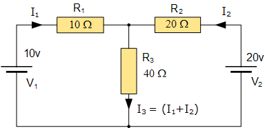
Example: Two-Mesh Circuit
Consider a circuit with two meshes:
- Mesh 1: Contains resistors R₁ and R₂ and voltage source V₁.
- Mesh 2: Contains resistors R₂ and R₃ and voltage source V₂.
The KVL equations are:
Practical Considerations
When dealing with dependent sources or non-linear elements, additional constraints must be incorporated. Supermeshes may be required if a current source is shared between two meshes.
Matrix Representation
For complex circuits, the system of KVL equations can be expressed in matrix form:
where Rᵢⱼ represents the total resistance in mesh i (if i = j) or the mutual resistance between meshes i and j (if i ≠ j).
2.4 Solving the System of Equations
Once the mesh equations are formulated using Kirchhoff’s Voltage Law (KVL), the next step is solving the resulting system of linear equations. For a circuit with N meshes, this system consists of N equations with N unknown mesh currents. The general form of these equations is:
Here, Rii represents the total resistance in mesh i, while Rij (where i ≠ j) denotes the mutual resistance shared by meshes i and j. Vi is the net voltage rise from sources in mesh i.
Matrix Representation
The system can be compactly expressed in matrix form as:
where R is the N×N resistance matrix, I is the column vector of mesh currents, and V is the column vector of source voltages. Solving for I yields:
Step-by-Step Solution Methods
1. Gaussian Elimination
This method systematically eliminates variables to reduce the system to upper triangular form. The steps are:
- Forward Elimination: Subtract multiples of equations to zero out coefficients below the diagonal.
- Back Substitution: Solve for unknowns starting from the last equation.
2. Cramer’s Rule
For small systems (N ≤ 3), Cramer’s Rule provides a direct solution:
where Rk is the matrix formed by replacing the k-th column of R with V.
3. Numerical Methods (for Large Systems)
For circuits with many meshes (N > 5), iterative methods like the Gauss-Seidel or Conjugate Gradient are preferred due to computational efficiency.
Practical Example
Consider a two-mesh circuit with:
Using matrix inversion:
Computational Tools
Engineers often leverage software like MATLAB, SPICE, or Python’s numpy.linalg.solve for large-scale systems. For example, in Python:
import numpy as np
R = np.array([[10, -4], [-4, 8]])
V = np.array([12, 0])
I = np.linalg.solve(R, V)
print(I)  # Output: [1.5, 0.75]
3. Circuits with Current Sources
3.1 Circuits with Current Sources
Handling Current Sources in Mesh Analysis
Current sources introduce constraints that simplify mesh analysis by directly defining the current in a particular branch. Unlike voltage sources, which contribute to the mesh equations via potential differences, current sources enforce a known current, reducing the number of independent equations needed.
Consider a circuit with a current source IS between two meshes. The current source imposes the condition:
where Im1 and Im2 are the mesh currents. This constraint allows one mesh current to be expressed in terms of the other, reducing the system of equations.
Supermesh Formation
When a current source lies between two meshes and is not shared with the outer loop, a supermesh must be formed. A supermesh combines the two meshes into a single larger loop, excluding the current source branch. The steps are:
- Identify the meshes sharing the current source.
- Exclude the current source branch and write a KVL equation for the combined loop.
- Add the current source constraint as an auxiliary equation.
For example, in a two-mesh circuit with a current source IS between meshes 1 and 2:
with the constraint:
Example: Circuit with Dependent Current Source
Dependent current sources require additional care. Suppose a circuit contains a current-controlled current source (CCCS) I = k Ix, where Ix is a branch current. The analysis proceeds as follows:
- Express Ix in terms of mesh currents.
- Substitute the dependent source relationship into the mesh equations.
- Solve the reduced system.
For a CCCS I = 2 I_{m1} in parallel with R2, the supermesh equation becomes:
Practical Considerations
In real-world circuits, current sources often model active components like transistors or operational amplifiers. For instance, a BJT in active mode approximates a current source between collector and emitter, simplifying small-signal analysis using mesh methods.
Non-ideal current sources with finite parallel resistance (Rp) can be converted to Thévenin equivalents if needed, though mesh analysis remains applicable by treating Rp as part of the mesh resistances.
3.2 Supermesh Formation
When analyzing circuits with current sources shared between two meshes, standard mesh analysis becomes cumbersome due to the undefined voltage drop across an ideal current source. A supermesh is a computational construct that simplifies such cases by combining the affected meshes into a single analytical entity while enforcing the current source constraint.
Conditions for Supermesh Creation
A supermesh is formed under the following conditions:
- A current source (dependent or independent) lies on the boundary of two meshes.
- The current source is not shared with the outer loop of the entire circuit.
Mathematical Derivation
Consider two meshes, i and j, sharing a current source Is. The mesh equations for the original meshes are:
Here, Vs represents the undefined voltage across the current source. Adding these equations eliminates Vs:
The system is then solved by supplementing this equation with the constraint imposed by the current source:
Step-by-Step Procedure
- Identify the meshes sharing the current source.
- Combine these meshes into a supermesh, excluding the branch containing the current source.
- Write the KVL equation for the supermesh.
- Add the current source constraint relating the mesh currents.
- Solve the system of equations for the unknown mesh currents.
Practical Example
Analyze the following circuit (described textually): A 10V voltage source connects to a 2Ω resistor in series with a 3A current source, which is shared between Mesh 1 (left loop) and Mesh 2 (right loop). Mesh 2 also includes a 4Ω resistor.
The supermesh equation (combining Meshes 1 and 2) is:
The current source imposes:
Solving these yields I1 = 3.67A and I2 = 0.67A.
Applications and Limitations
Supermeshes are indispensable in:
- Power supply networks with parallel regulator circuits.
- Transistor amplifier biasing networks with current mirrors.
However, they cannot resolve circuits where:
- Current sources form part of the circuit's outer loop.
- Non-planar networks prevent clear mesh identification.
3.3 Dependent Sources in Mesh Analysis
Dependent sources introduce additional constraints in mesh analysis, requiring careful handling to maintain consistency in the system of equations. Unlike independent sources, which provide fixed voltage or current values, dependent sources are functions of other circuit variables, such as branch currents or node voltages.
Types of Dependent Sources
Four primary dependent sources exist:
- Voltage-controlled voltage source (VCVS): Output voltage depends on another voltage in the circuit.
- Current-controlled voltage source (CCVS): Output voltage depends on a current elsewhere in the circuit.
- Voltage-controlled current source (VCCS): Output current depends on another voltage.
- Current-controlled current source (CCCS): Output current depends on another current.
Modified Mesh Analysis Procedure
When dependent sources are present, the standard mesh analysis procedure expands:
- Assign mesh currents as usual, labeling them \( I_1, I_2, \dots, I_n \).
- Write the constitutive equations for all dependent sources in terms of mesh currents.
- Apply Kirchhoff's voltage law (KVL) to each mesh, treating dependent sources initially as independent sources.
- Substitute the dependent source expressions into the KVL equations.
- Solve the resulting system of equations for the mesh currents.
Example: CCVS in a Two-Mesh Circuit
Consider a circuit with two meshes where Mesh 1 contains an independent voltage source \( V_s \) and resistor \( R_1 \), and Mesh 2 contains resistor \( R_2 \) and a CCVS with strength \( r \) controlling current \( I_1 \). The KVL equations become:
Rearranging terms yields the matrix equation:
Practical Considerations
Dependent sources frequently appear in transistor small-signal models (VCCS in MOSFETs) and operational amplifier circuits (VCVS). In SPICE simulations, proper implementation requires:
- Correctly identifying the controlling variable
- Ensuring the dependent source doesn't create impossible constraints (e.g., zero-resistance current sources)
- Verifying dimensional consistency in gain factors (e.g., \( r \) has units of ohms for CCVS)
Numerical Stability
Circuits with dependent sources may exhibit:
- Singular matrices if the dependent source creates a degenerate case
- Numerical sensitivity when gain factors approach very large values
- Need for iterative solutions in nonlinear dependent source cases
Modern circuit simulators handle these cases through:
- Modified nodal analysis with supplemental equations
- Automatic scaling of variables
- Advanced linear algebra techniques for ill-conditioned matrices
4. Analyzing a Simple Resistive Circuit
4.1 Analyzing a Simple Resistive Circuit
Fundamentals of Mesh Analysis
Mesh analysis is a systematic method for determining currents in planar circuits by applying Kirchhoff's Voltage Law (KVL) to closed loops (meshes). The technique simplifies circuit analysis by reducing the number of equations needed compared to nodal analysis, particularly in circuits with many series-connected components.
For a circuit with N meshes, we write N independent KVL equations. Each equation accounts for voltage drops across resistors and rises due to sources within the mesh. The resulting system of linear equations can be solved for the mesh currents, from which branch currents are derived.
Step-by-Step Derivation for a Two-Mesh Circuit
Consider the following DC resistive circuit with two meshes:
Let mesh current I1 flow clockwise in the left mesh and I2 in the right mesh. Applying KVL to each mesh:
Rearranging terms gives the matrix equation:
Practical Considerations and Computational Efficiency
For circuits with n meshes, the resistance matrix exhibits symmetry about the diagonal (Rij = Rji). This property allows optimization in numerical solvers. The computational complexity scales as O(n3) for direct matrix inversion, though sparse matrix techniques can improve performance for large networks.
In experimental settings, mesh analysis proves particularly valuable for:
- Troubleshooting power distribution networks
- Analyzing voltage regulator circuits
- Designing active filter stages
Supermesh Technique for Current Sources
When a current source exists between two meshes, we create a supermesh by excluding the current source branch. The analysis proceeds with:
- KVL around the supermesh perimeter
- An auxiliary equation relating the mesh currents to the source current
For example, if a current source IS flows from Mesh 1 to Mesh 2:
This constraint equation replaces one of the standard mesh equations in the system.
4.2 Mesh Analysis in AC Circuits
Mesh analysis extends naturally to AC circuits, where impedances replace resistances, and phasor representations simplify sinusoidal steady-state analysis. The method remains systematic but requires handling complex numbers due to reactive components (inductors and capacitors).
Phasor Representation and Impedance
In AC circuits, voltages and currents are represented as phasors, transforming time-domain differential equations into algebraic equations in the frequency domain. The impedance Z of an element is given by:
where R is resistance, X is reactance (XL = ωL for inductors, XC = -1/ωC for capacitors), and j is the imaginary unit.
Steps for Mesh Analysis in AC Circuits
- Convert sources to phasor form: Express all sinusoidal sources as phasors (e.g., v(t) = Vmcos(ωt + ϕ) becomes V = Vm∠ϕ).
- Represent impedances: Replace resistors, inductors, and capacitors with their respective impedances.
- Assign mesh currents: Define clockwise or counterclockwise mesh currents (I1, I2, ..., In).
- Apply Kirchhoff’s Voltage Law (KVL): Write KVL equations for each mesh, summing voltage drops across impedances and sources.
- Solve the system of equations: Use matrix methods or substitution to solve for the mesh currents in complex form.
- Convert back to time domain (if needed): Transform phasor currents to their time-domain expressions.
Example: Two-Mesh AC Circuit
Consider a circuit with two meshes:
- Mesh 1: Voltage source V1 = 10∠0° V, impedance Z1 = 5 + j3 Ω.
- Mesh 2: Impedance Z2 = 2 - j4 Ω, shared branch impedance Z12 = j5 Ω.
The mesh equations are:
Substituting values:
Simplifying:
Solving this system yields the phasor currents I1 and I2.
Practical Considerations
Mesh analysis in AC circuits is widely used in:
- Power systems: Analyzing transmission lines and load flow.
- Filter design: Determining frequency response of RLC networks.
- Impedance matching: Optimizing power transfer in RF circuits.
Complex arithmetic can be error-prone, so computational tools (SPICE, MATLAB) are often employed for verification.
4.3 Real-world Engineering Applications
Power Distribution Networks
Mesh analysis is extensively used in three-phase power systems to model and analyze balanced and unbalanced loads. In a distribution network with multiple loops, Kirchhoff’s Voltage Law (KVL) applied via mesh currents simplifies the calculation of branch currents and voltage drops. For example, consider a three-wire system with impedances Z1, Z2, Z3:
Here, Zii represents self-impedances, and Zij (i ≠ j) denotes mutual impedances. Solving this matrix equation yields mesh currents, which directly translate to line currents in delta or wye configurations.
Integrated Circuit Design
In VLSI, mesh analysis aids in modeling power/ground grids to minimize IR drop and electromigration. A typical grid with n nodes and m branches can be reduced to a sparse impedance matrix. For a unit cell with resistance R and current source I0:
SPICE-based solvers exploit mesh analysis to simulate parasitic effects, ensuring signal integrity in high-speed designs like DDR5 interfaces.
Electromagnetic Compatibility (EMC)
To predict crosstalk in multi-conductor transmission lines, mesh formulations model mutual inductance (Lm) and capacitance (Cm). For two adjacent traces:
This approach is critical in PCB design for minimizing EMI in automotive CAN buses or aerospace avionics.
Renewable Energy Systems
In photovoltaic arrays, mesh analysis evaluates mismatch losses due to partial shading. A 4×4 panel matrix with bypass diodes can be represented as:
where Iph,k is the photocurrent and Im,k the mesh current of the k-th cell. This identifies hotspots and optimizes MPPT algorithms.
Biomedical Instrumentation
Mesh methods model bioimpedance networks in EEG/ECG electrodes. For a tetra-polar impedance measurement:
This isolates tissue impedance from electrode-skin interface artifacts, improving diagnostic accuracy in impedance cardiography.
5. Sign Conventions and Errors
5.1 Sign Conventions and Errors
Mesh analysis relies on consistent sign conventions to ensure accurate current and voltage calculations. A misapplied sign can propagate errors throughout the entire circuit solution. The two primary conventions are the passive sign convention and the active sign convention, which dictate how voltage polarities and current directions are assigned.
Passive Sign Convention
In the passive sign convention, current is considered positive when it enters the positive terminal of a component. For resistors, this aligns with Ohm's Law:
For voltage sources, the polarity is explicitly defined, and the mesh current direction determines the sign of the voltage drop. If the current flows from the negative to the positive terminal, the voltage source contributes positively to the mesh equation.
Active Sign Convention
Active elements, such as dependent sources, require careful handling. A current-controlled voltage source (CCVS), for example, introduces a voltage proportional to a branch current:
where rm is the transresistance and Ix is the controlling current. The sign depends on the relative orientation of the controlling current and the dependent source's polarity.
Common Sign Errors
Three frequent mistakes in mesh analysis include:
- Inconsistent current direction: If mesh currents are not uniformly defined (e.g., clockwise vs. counterclockwise), voltage drops may be incorrectly summed.
- Misaligned voltage polarities: Voltage sources opposing the assumed current direction must be treated as negative contributions.
- Dependent source misassignment: Failing to account for the controlling variable's direction leads to incorrect dependent source terms.
Practical Example: Dual-Mesh Circuit
Consider a circuit with two meshes and a shared current source. The mesh equations are:
Here, V2 is negative because its polarity opposes the assumed mesh current I2. A sign error in the second equation would invert the solution.
Verification Techniques
To minimize errors:
- Cross-validate with Kirchhoff’s Voltage Law (KVL): Ensure the sum of voltage drops around each mesh matches the applied sources.
- Use simulation tools: SPICE-based analyzers can quickly identify discrepancies in hand calculations.
- Dimensional analysis: Verify that derived currents and voltages have physically plausible units and magnitudes.
In high-frequency or nonlinear circuits, additional considerations arise due to parasitic elements and non-ideal component behavior, but the core sign conventions remain foundational.
5.2 Incorrect Mesh Identification
Mesh analysis relies on correctly identifying independent meshes in a circuit. A common pitfall arises when meshes are improperly defined, leading to incorrect equations and invalid solutions. This occurs primarily in two scenarios: non-planar circuits and redundant mesh selection.
Non-Planar Circuits and Mesh Ambiguity
A circuit is planar if it can be drawn on a plane without any intersecting branches. Non-planar circuits, such as those with crossovers (e.g., bridges or 3D interconnects), cannot be analyzed using standard mesh analysis without modification. Attempting to force mesh currents in such cases results in:
- Overdefined systems: More mesh equations than independent loops exist.
- KVL violations: Incorrect summation of voltage drops due to misassigned current paths.
For example, consider a Wheatstone bridge with a cross-branch resistor. If meshes are drawn without accounting for the non-planarity, the resulting equations will conflict with Kirchhoff's laws.
Redundant Mesh Selection
Even in planar circuits, selecting meshes that are not independent introduces errors. A mesh is independent if its equation cannot be derived from a linear combination of other mesh equations. Redundancy occurs when:
- Two meshes share all their branches (supermesh errors).
- An outer loop is mistakenly included alongside inner loops.
Violating this rule leads to a rank-deficient matrix in the mesh equation system, rendering it unsolvable.
Practical Implications
Incorrect mesh identification manifests in simulation tools (e.g., SPICE) as convergence failures or nonsensical current values. For example, LTspice may return singular matrix warnings if mesh equations are linearly dependent. Debugging requires:
- Verifying planarity using graph theory (e.g., Kuratowski's theorem).
- Counting branches and nodes to confirm the correct number of meshes.
- Using loop analysis as a fallback for non-planar topologies.
Case Study: Dual-Power-Supply Circuit
A common error occurs in circuits with multiple voltage sources. If two meshes are defined such that both include the same source branch, their equations become coupled incorrectly. The correct approach isolates each source within a single mesh or uses supermesh techniques.
Here, V1 and V2 must belong to distinct meshes. Merging them into one mesh would eliminate the independent equation for I2.
5.3 Numerical Solution Techniques
Mesh analysis reduces complex circuits to a system of linear equations, solvable through matrix methods. For a network with N meshes, Kirchhoff's Voltage Law (KVL) yields N independent equations of the form:
where Rik represents the resistance common to meshes i and k, Ik is the mesh current, and Vi is the net voltage source in mesh i. The system is expressed in matrix form as RI = V, where R is the resistance matrix, I is the current vector, and V is the voltage vector.
Matrix Formulation and Solution
The resistance matrix R is symmetric for linear passive networks, with diagonal elements Rii representing the sum of resistances in mesh i, and off-diagonal elements Rik (where i ≠ k) denoting the negative of shared resistances. For a 3-mesh circuit:
Solutions are obtained via:
- Direct methods (e.g., Gaussian elimination) for small systems.
- Iterative methods (e.g., Jacobi, Gauss-Seidel) for large sparse matrices.
- Matrix inversion (I = R−1V), though computationally intensive for N > 4.
Computational Efficiency
Sparse matrix techniques exploit zero entries in R to reduce storage and operations. For example, in a mesh with no shared components between loops i and j, Rij = 0. Algorithms like LU decomposition with partial pivoting improve numerical stability for ill-conditioned matrices.
Practical Implementation
Modern circuit simulators (e.g., SPICE) use modified nodal analysis, but mesh methods remain valuable for:
- Power distribution networks, where loop currents correlate with physical branch currents.
- Fault analysis, identifying current distributions during short circuits.
- Educational tools, reinforcing KVL through systematic equation construction.
Case Study: Nonplanar Circuits
For nonplanar topologies (e.g., circuits requiring a crossing without intersection), mesh analysis extends by introducing virtual cuts or switching to nodal methods. The resistance matrix loses symmetry if dependent sources are present, requiring careful adjustment of off-diagonal terms.
where β accounts for source coupling. Numerical solvers must handle such asymmetries to avoid convergence issues.
6. Recommended Textbooks
6.1 Recommended Textbooks
- Network Analysis and Synthesis - O'Reilly Media — 2.2 Mesh Analysis; 2.3 Nodal Analysis; 2.4 Super Nodal Analysis; 2.5 Super Mesh Analysis; 2.6 Methods of Solving Complex Network Problems. 2.6.1 Numerical Problems Based on Kirchhoff's Laws; 2.6.2 Numerical Problems Based on Mesh and Nodal Analysis; Review Questions; Multiple Choice Questions; Answers; 3. Steady State Analysis of AC Circuits
- Practical Electronics/Circuits Analysis/Mesh Analysis — A caveat: mesh analysis can only be used on 'planar' circuits (i.e. there are no crossed, but unconnected, wires in the circuit diagram.) Steps: 1. Draw circuit in planar form (if possible.) 2. Identify meshes and name mesh currents. Mesh currents should be in the clockwise direction.
- Readings | Introductory Analog Electronics Laboratory | Electrical ... — This section provides the list of textbooks for the course and the schedule of readings for the lecture sessions. ... Jimmie J. Schaum's Outlines Electronic Devices and Circuits. 2nd ed. New York, NY: McGraw-Hill, 2002. ISBN: 9780071362702. ... graphical analysis Neamen 5.2 to 5.2.3 and 5.3.3, J&J pp. 216-220, Cathey 3.6 to 3.7. D. Common ...
- The Best Online Library of Electrical Engineering Textbooks — Electronics textbooks including: Fundamentals of Electrical Engineering, Electromagnetics, Introduction to Electricity, Magnetism, & Circuits and more. ... Mesh Analysis 7.1; Superposition Theorem 7.2; Thévenin's Theorem 7.3; ... both this textbook and the Circuits 101 tutorials will provide two different methods of teaching and it is highly ...
- Mesh-Current and Node-Voltage Analysis - O'Reilly Media — 6 Mesh-Current and Node-Voltage Analysis OBJECTIVES In this chapter you will learn about: Matrices and determinants Solution of simultaneous equations using determinants Gauss elimination technique Network analysis by mesh currents … - Selection from Electrical Technology, Volume 1 [Book]
- PDF MITx 6.002.1x Circuits and Electronics I: Basic Circuit Analysis — 3. Textbook The course textbook is the following: Foundations of Analog and Digital Electronic Circuits. Agarwal, Anant, and Jeffrey H. Lang. San Mateo, CA: Morgan Kaufmann Publishers, Elsevier, July 2005. ISBN: 9781558607354. The textbook (physical or ebook) may be purchased from Elsevier.
- 6.1: Introduction - Engineering LibreTexts — Nodal analysis is the most general technique and can be applied to virtually any circuit. Mesh analysis is nearly as versatile and works well if only voltage sources are present. Both analysis methods generate a system of simultaneous linear equations that are used to solve the circuit for desired voltages or currents.
- 6: Nodal and Mesh Analysis - Engineering LibreTexts — The LibreTexts libraries are Powered by NICE CXone Expert and are supported by the Department of Education Open Textbook Pilot Project, the UC Davis Office of the Provost, the UC Davis Library, the California State University Affordable Learning Solutions Program, and Merlot. We also acknowledge previous National Science Foundation support ...
- AC Electrical Circuit Analysis: A Practical Approach + Lab Manual — About the book An essential and practical text for both students and teachers of AC electrical circuit analysis, this text picks up where the companion DC electric circuit analysis text leaves off. Beginning with basic sinusoidal functions, ten chapters cover topics including series, parallel, and series-parallel RLC circuits. Numerous theorems […]
6.2 Online Resources and Tutorials
- Linear Circuits 1: DC Analysis - Coursera — 3.1 Lab Demo: Electrical Components • 6 minutes • Preview module; 3.2 Lab Demo: Basic Circuits • 6 minutes; 3.3 Mesh Analysis. • 10 minutes 3.4 Node Analysis. • 8 minutes Sample Problem: Mesh/Node (Supernode) • 10 minutes Sample Problem: Mesh Analysis (Super Mesh) • 10 minutes Sample Problem: Mesh Analysis (Depend Sources) 1 • 6 minutes; Sample Problem: Mesh Analysis (Depend ...
- 6: Nodal and Mesh Analysis - Engineering LibreTexts — This page titled 6: Nodal and Mesh Analysis is shared under a CC BY-NC-SA 4.0 license and was authored, remixed, and/or curated by James M. Fiore via source content that was edited to the style and standards of the LibreTexts platform.
- Mesh Analysis | EE281 - Electric Circuits - ozank.gitbooks.io — Mesh Analysis. In the Mesh analysis the unknown parameters are mesh currents instead of the node voltages. A mesh is a loop which does not contain any other loops within it. In the Nodal analysis we have used Kirchhoff's Current Law, in the Mesh Analysis Kirchoof's Voltage Law will be used.
- 6.3: Mesh Analysis - Engineering LibreTexts — Mesh analysis is similar to nodal analysis in that it can handle complex multi-source circuits. In some ways it is the mirror image of nodal analysis. While nodal analysis uses Kirchhoff's current law to create a series of current summations at various nodes, mesh analysis uses Kirchhoff's voltage law to create a series of loop equations that ...
- 7.1 Mesh Analysis - University of Saskatchewan — Calculating Current by the Mesh Analysis Approach. Find the currents flowing in the circuit in Figure 7.1.1. (Figure 7.1.1) Figure 7.1.1 This circuit is a combination of series and parallel configurations of resistors and voltage sources. Redrawn from Figure 6.3.11, with current loops drawn for the purpose of mesh analysis. Strategy
- 6.1: Introduction - Engineering LibreTexts — Nodal analysis is the most general technique and can be applied to virtually any circuit. Mesh analysis is nearly as versatile and works well if only voltage sources are present. Both analysis methods generate a system of simultaneous linear equations that are used to solve the circuit for desired voltages or currents.
- Integrated Optomechanical Analysis, Second Edition - SPIE Digital Library — This edition updates and expands the content in the original SPIE Tutorial Text to include new illustrations and examples, as well as chapters about structural dynamics, mechanical stress, superelements, and the integrated optomechanical analysis of a telescope and a lens assembly.
- Mesh Analysis for Circuits Explained - YouTube — This tutorial introduces Mesh Analysis and explains how to use it to solve unknowns in circuits. I find it helpful to label on unknown branch currents before...
- Basic Meshing for Structural Simulation Using Ansys Mechanical - Ansys ... — Introducing Ansys Electronics Desktop on Ansys Cloud. The Watch & Learn video article provides an overview of cloud computing from Electronics Desktop and details the product licenses and subscriptions to ANSYS Cloud Service that are...
- Learning Center - COMSOL — Learn how to use COMSOL Multiphysics® for specific application areas. Browse the COMSOL Learning Center for self-paced courses and articles.
6.3 Advanced Topics in Circuit Analysis
- Linear Circuits 1: DC Analysis - Coursera — 3.1 Lab Demo: Electrical Components • 6 minutes • Preview module; 3.2 Lab Demo: Basic Circuits • 6 minutes; 3.3 Mesh Analysis. • 10 minutes 3.4 Node Analysis. • 8 minutes Sample Problem: Mesh/Node (Supernode) • 10 minutes Sample Problem: Mesh Analysis (Super Mesh) • 10 minutes Sample Problem: Mesh Analysis (Depend Sources) 1 • 6 minutes; Sample Problem: Mesh Analysis (Depend ...
- 6: Nodal and Mesh Analysis - Engineering LibreTexts — Electronics AC Electrical Circuit Analysis: A Practical Approach (Fiore) 6: Nodal and Mesh Analysis Expand/collapse global location 6: Nodal and Mesh Analysis ... This page titled 6: Nodal and Mesh Analysis is shared under a CC BY-NC-SA 4.0 license and was authored, remixed, ...
- 6.3: Mesh Analysis - Engineering LibreTexts — Therefore there are circuits that cannot be solved using mesh. Consider the circuit of Figure \(\PageIndex{1}\). This circuit has two voltage sources and cannot be simplified further, although it can be solved using either superposition or nodal analysis. For mesh analysis, we begin by designating a set of current loops.
- Mesh Analysis for ac Circuits - realnfo.com — Before examining the application of the method to ac networks, the student should first review the appropriate sections on mesh analysis in Chapter 6 since the content of this section will be limited to the general conclusions of Chapter 6. The general approach to mesh analysis for independent sources includes the same sequence of steps appearing in Chapter 6.
- PDF DC Electrical Circuit Analysis - mvcc.edu — continues with chapters covering network theorems, more advanced techniques such as nodal and mesh analysis, and finally finishes with introductions to capacitors, inductors and magnetic circuits. The companion AC Electrical Circuit Analysis text picks up after this point. Each chapter begins with a set of learning objectives
- 7 Advanced Circuit Analysis Techniques - Introduction to Electricity ... — In this case, you could solve the circuit in Figure 7.0.1(a) by direct application of the Mesh Analysis technique. But this solution requires solving four simultaneous equations for the four loops in the circuit, and you may not have a computer handy, and may not be inclined to solve the linear system by hand.
- Mesh Analysis with Current Sources - Realnfo — Applying mesh analysis to circuits containing current sources (dependent or independent) may appear complicated. ... Because mesh analysis applies KVL—which requires that we know the voltage across each branch—and we do not know the voltage across a current source in advance. However, a supermesh must satisfy KVL like any other mesh ...
- Mesh Analysis | EE281 - Electric Circuits - ozank.gitbooks.io — Mesh analysis can only be applied to planar circuit. A planar circuit can be drawn with no branches crossing one another. ... Label each mesh in the circuit. Write KVL equations for each mesh. Solve equations for the mesh currents. Things to be careful: Although, the direction of mesh currents (clockwise or counterclockwise) is arbitrary, and ...
- Mesh Analysis - Electrical Engineering Textbooks | CircuitBread — Draw mesh current loops, ensuring: . each loop is unique; and; all circuit elements—voltage sources, resistors, capacitors, inductors, etc. and short circuits—are covered by at least one loop. Apply loop rule as described in Kirchhoff's Rules (particularly with reference to Figure 6.3.5) and solve simultaneous equations.; Add or subtract mesh currents in branches that are covered by ...
- Circuit Theory - Wikibooks, open books for an open world — Toggle Circuit Analysis Tips and Tricks subsection. 6.1 Impedance, Node, Mesh. 6.2 Source Transformation. 6.3 Tips and Tricks. 7 Transient Response. 8 State Variables. 9 Filters. 10 Control. 11 Power. Toggle the table of contents. ... and will not stop to explain the fundamental topics in Calculus. This book shows where Laplace transforms ...
Related Circuits
 /var/www/html/nextgr/view-tutorial.php on line 513
Deprecated: htmlspecialchars(): Passing null to parameter #1 ($string) of type string is deprecated in /var/www/html/nextgr/view-tutorial.php on line 513
"> Bricolage YumYum
Schematics map the everyday. Our mundane yet gingerly interactions are inundated by the electronic, constituted by the digital and the analog. Circuitry is the river system for the daily task of manipulating and reproducing society. It is the undisputed bedrock of contemporary social mediation. Conductors, resistors, current, voltage, amps, Ohms...
 /var/www/html/nextgr/view-tutorial.php on line 513
Deprecated: htmlspecialchars(): Passing null to parameter #1 ($string) of type string is deprecated in /var/www/html/nextgr/view-tutorial.php on line 513
"> Mesh Current Analysis - DC Circuit Theory
Electronics Tutorial about Mesh Current Analysis and Mesh Analysis Examples used to Analyse Complex Electrical Circuits in DC Theory..