Mutual Inductance
1. Definition and Basic Principles
Mutual Inductance: Definition and Basic Principles
Mutual inductance describes the phenomenon where a changing current in one circuit induces an electromotive force (EMF) in a nearby circuit due to magnetic coupling. The fundamental principle arises from Faraday's Law of Induction and is quantified by the mutual inductance coefficient M.
Mathematical Formulation
Consider two circuits, labeled 1 and 2. The mutual inductance M21 is defined as the ratio of the magnetic flux Φ21 through circuit 2 due to the current I1 in circuit 1:
where N2 is the number of turns in circuit 2. By reciprocity, M12 = M21 = M, meaning the mutual inductance between two circuits is symmetric.
Derivation from Faraday's Law
The induced EMF in circuit 2 due to a time-varying current in circuit 1 is given by:
This shows that the induced voltage is proportional to the rate of change of current in the primary circuit. The negative sign reflects Lenz's Law, indicating the induced EMF opposes the change in current.
Coefficient of Coupling
The mutual inductance between two circuits depends on their geometry and the medium between them. The coupling coefficient k (0 ≤ k ≤ 1) relates mutual inductance to the self-inductances L1 and L2:
For perfect coupling (k = 1), all magnetic flux generated by one circuit links the other. In practice, k is less than 1 due to leakage flux.
Practical Applications
Mutual inductance is the operating principle behind transformers, wireless power transfer systems, and inductive sensors. In RF engineering, mutual coupling between transmission lines or antennas can lead to desired (e.g., directional couplers) or undesired (e.g., crosstalk) effects.
The energy stored in a system of two magnetically coupled circuits is:
where the sign depends on whether the magnetic fields aid or oppose each other.
Relationship Between Self-Inductance and Mutual Inductance
The relationship between self-inductance (L) and mutual inductance (M) is fundamental in the analysis of coupled inductors, transformers, and other electromagnetic systems. The coupling between two coils is quantified by the mutual inductance, while their individual energy storage capabilities are described by their self-inductances.
Mathematical Derivation of Coupling Coefficient
The coupling coefficient (k) defines the extent of magnetic linkage between two inductors and is derived from their mutual and self-inductances. For two coils with inductances L1 and L2, the mutual inductance M is bounded by:
where k ranges from 0 (no coupling) to 1 (perfect coupling). This relationship arises from the magnetic flux linkage between the coils. If a current I1 flows through the first coil, the induced voltage in the second coil is:
Similarly, the self-induced voltage in the first coil is:
Energy Considerations in Coupled Inductors
The total energy stored in a system of two coupled inductors is given by:
The sign of the mutual inductance term depends on the relative winding directions (dot convention). For additive coupling (flux aiding), the term is positive; for subtractive coupling (flux opposing), it is negative.
Practical Implications and Applications
In transformer design, maximizing k ensures efficient energy transfer. Tightly coupled coils (k ≈ 1) are used in power transformers, while loosely coupled coils (k < 0.5) appear in tuned circuits and wireless power transfer systems. The leakage inductance, given by:
quantifies the uncoupled portion of the magnetic field and is critical in high-frequency applications.
Case Study: Transformer Equivalent Circuit
A real transformer can be modeled using an ideal transformer with leakage inductances and parasitic elements. The mutual inductance M and self-inductances L1, L2 define the turns ratio (N1/N2):
This approximation holds when k is close to unity, but deviations occur due to non-ideal coupling.
1.3 The Dot Convention in Mutual Inductance
The dot convention is a standardized method for indicating the relative polarity of mutually coupled inductors in circuit diagrams. It resolves ambiguities in the sign of the mutual inductance term M when analyzing circuits with magnetic coupling. The convention is essential for correctly predicting the behavior of transformer-coupled networks, coupled filters, and other magnetically linked systems.
Mathematical Foundation
The voltage induced in one coil due to current changes in another is given by:
where the ± sign depends on the winding orientation. The dot convention provides a systematic way to determine whether mutual inductance terms add or subtract.
Rules of the Dot Convention
- Current entering a dotted terminal induces a positive voltage at the other coil's dotted terminal
- Current entering an undotted terminal induces a negative voltage at the other coil's undotted terminal
- The mutual inductance M is always positive - the sign is determined by the dot placement
Practical Implementation
Consider two mutually coupled inductors with dots on one end of each coil. When analyzing the circuit:
- Define current directions (entering or leaving dotted terminals)
- Apply Faraday's law of induction
- Use the dot convention to determine the sign of mutual inductance terms
For example, if current i1 enters the dotted terminal of coil 1 and current i2 leaves the dotted terminal of coil 2, the voltage equations become:
Visual Representation
Advanced Applications
In three-phase transformer banks, the dot convention becomes critical for proper phase relationships. Power engineers use extended dot notation to indicate:
- Wye-delta phase shifts
- Zero-sequence current paths
- Parasitic capacitance effects in high-frequency transformers
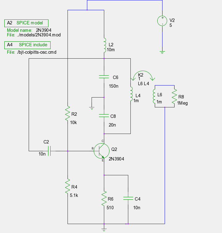
For coupled transmission lines, the convention helps predict crosstalk and modal propagation characteristics. Modern circuit simulators like SPICE implement the dot convention through the coupling coefficient K in their mutual inductance models.
Historical Context
The dot notation was formalized in the early 20th century as telephone systems required precise analysis of transformer-coupled circuits. Oliver Heaviside's work on operational methods provided the theoretical foundation, while practical implementation standards were developed by Bell Labs engineers.
2. Mutual Inductance Formula and Derivation
2.1 Mutual Inductance Formula and Derivation
Mutual inductance (M) quantifies the magnetic coupling between two coils, describing how a changing current in one coil induces a voltage in another. The phenomenon is governed by Faraday's Law of Induction and the Biot-Savart Law, linking magnetic flux to induced electromotive force (EMF).
Fundamental Definition
The mutual inductance between two circuits (1 and 2) is defined as the ratio of the magnetic flux (Φ12) through circuit 2 due to the current (I1) in circuit 1:
where N2 is the number of turns in coil 2. By reciprocity, M21 = M12, simplifying analysis.
Derivation from First Principles
Starting with Faraday's Law, the induced EMF (ε2) in coil 2 due to a time-varying current in coil 1 is:
The magnetic flux Φ12 is proportional to I1 via the mutual inductance:
Substituting into Faraday's Law and differentiating yields:
This confirms M as the proportionality constant linking the rate of current change in coil 1 to the induced voltage in coil 2.
Neumann’s Formula for Mutual Inductance
For arbitrary coil geometries, Neumann’s formula provides a general expression:
where μ0 is the permeability of free space, dl1 and dl2 are infinitesimal segments of coils 1 and 2, and r is the distance between them. This double line integral accounts for all geometric dependencies.
Practical Example: Two Solenoids
For two coaxial solenoids (length l, radii r1 and r2, turns N1 and N2), mutual inductance simplifies to:
assuming r1 ≤ r2 and perfect flux linkage. Leakage flux reduces M in real systems.
Applications and Implications
- Transformers: Mutual inductance enables energy transfer between primary and secondary windings.
- Wireless Power Transfer: Resonant inductive coupling relies on optimized M for efficiency.
- Cross-Talk in Circuits: Unwanted mutual inductance between traces can degrade signal integrity.
Understanding M is critical for designing inductive systems, minimizing interference, and maximizing energy coupling efficiency.
2.2 Coupling Coefficient and Its Significance
Definition and Mathematical Formulation
The coupling coefficient (k) quantifies the degree of magnetic linkage between two inductively coupled circuits. It is a dimensionless parameter bounded between 0 (no coupling) and 1 (perfect coupling). The coupling coefficient is derived from the mutual inductance (M) and the self-inductances (L1 and L2) of the two coils:
This equation highlights that k depends on the geometric arrangement and magnetic permeability of the medium. For tightly wound coils with overlapping magnetic flux, k approaches unity, whereas loosely coupled systems exhibit lower values.
Physical Interpretation
The coupling coefficient directly influences energy transfer efficiency between coupled inductors. In an ideal transformer, k = 1 ensures maximum power transfer with minimal leakage flux. Practical systems, however, face constraints due to:
- Leakage inductance: Flux not shared between coils reduces k.
- Core material saturation: Nonlinear permeability limits achievable coupling.
- Geometric misalignment: Axial or angular displacement degrades k.
Measurement Techniques
Experimental determination of k involves:
- Inductance bridge methods: Measure L1, L2, and M under open- and short-circuit conditions.
- Resonant frequency shift: Observe frequency splitting in coupled LC tanks, where:
Practical Applications
The coupling coefficient is critical in:
- Wireless power transfer (WPT): High-k designs (>0.8) enable efficient resonant inductive coupling.
- Transformer design: Interleaved winding techniques maximize k to reduce eddy current losses.
- RF circuits: Directional couplers use controlled k for precise power splitting.
Case Study: Coupled Resonators in MRI
In magnetic resonance imaging (MRI), quadrature birdcage coils achieve k ≈ 0.7–0.9 to optimize signal-to-noise ratio while minimizing cross-talk. The coupling coefficient here is tuned by adjusting the overlap angle between adjacent rungs.
where N is the number of coil segments. This geometric dependence underscores the interplay between physical design and electromagnetic performance.
2.3 Mutual Inductance in Series and Parallel Circuits
Series Connection of Mutually Coupled Inductors
When two inductors with mutual inductance M are connected in series, their effective inductance depends on the relative orientation of their magnetic fields. The total inductance Ltotal is given by:
The sign of the mutual inductance term depends on whether the fluxes are aiding (+) or opposing (-). This arises from the voltage induced across each inductor due to mutual coupling:
In practical applications, such as transformer windings or coupled RF coils, the dot convention determines the sign of M. For aiding fluxes (dots on the same end), mutual inductance adds constructively. For opposing fluxes, it subtracts.
Parallel Connection of Mutually Coupled Inductors
For parallel-connected inductors with mutual coupling, the equivalent inductance becomes more complex due to circulating currents. The general form is:
Again, the sign depends on flux orientation. The derivation comes from solving the coupled voltage equations:
For identical inductors (L1 = L2 = L), this simplifies to:
Energy Considerations
The energy stored in coupled inductors reveals why M cannot exceed the geometric mean of L1 and L2:
Since energy cannot be negative, this imposes the condition M ≤ √(L1L2), defining the coupling coefficient k = M/√(L1L2).
Practical Implications
- Transformer design: Series aiding connections maximize inductance in flyback converters.
- Filter networks: Parallel combinations with controlled k create tuned circuits with specific bandwidths.
- Interference mitigation: Opposing series connections cancel stray inductance in high-speed PCB layouts.
In RF applications, mutual inductance enables impedance matching through inductive coupling, while in power systems, it governs fault current distribution in parallel busbars.
3. Transformers: Theory and Operation
Transformers: Theory and Operation
The operation of a transformer is fundamentally governed by the principles of mutual inductance, where energy is transferred between two or more magnetically coupled coils without a direct electrical connection. The primary and secondary windings share a common magnetic flux, enabling voltage transformation via Faraday's law of induction.
Ideal Transformer Model
An ideal transformer assumes no energy losses, infinite core permeability, and perfect magnetic coupling (k = 1). The voltage and current relationships are derived from the turns ratio N:
where a is the turns ratio, and subscripts p and s denote primary and secondary quantities, respectively. Power conservation holds (P_p = P_s) in this lossless model.
Real-World Non-Ideal Effects
Practical transformers exhibit:
- Leakage flux: Imperfect coupling (k < 1) causes flux not shared by both windings, modeled as series inductances.
- Core losses: Hysteresis and eddy currents in ferromagnetic materials dissipate energy.
- Winding resistance: Ohmic losses in copper windings.
- Magnetizing current: Finite core permeability requires current to establish flux.
Equivalent Circuit Model
The lumped-parameter model incorporates these effects:
Key components include:
- R_p, R_s: Primary and secondary winding resistances
- X_p, X_s: Leakage reactances
- R_c: Core loss resistance
- X_m: Magnetizing reactance
Transformer Efficiency and Regulation
Efficiency (η) and voltage regulation (%VR) are critical performance metrics:
where nl and fl denote no-load and full-load conditions. High-efficiency designs (>95%) are achieved through low-loss core materials and optimal winding geometry.
Three-Phase Transformer Configurations
For power systems, three-phase transformers use either:
- Bank of single-phase units
- Integrated three-phase core with wye (Y) or delta (Δ) connections
The line-to-line voltage transformation follows:
where the √3 factor arises from phase-to-line conversions in Y-Δ or Δ-Y configurations.
High-Frequency Transformers
In switched-mode power supplies, transformers operate at kHz-MHz frequencies. Key considerations include:
- Skin and proximity effects increasing AC resistance
- Core material selection for high-frequency operation (e.g., ferrite)
- Reduced size due to Faraday's law scaling with frequency
3.2 Inductive Coupling in Wireless Power Transfer
Mutual inductance forms the backbone of resonant inductive coupling, the dominant mechanism in mid-range wireless power transfer (WPT) systems. When two coils are brought into proximity, their magnetic fields interact, enabling energy transfer without physical contact. The efficiency of this coupling depends critically on the coupling coefficient k, defined as:
where M is the mutual inductance, and L1, L2 are the self-inductances of the primary and secondary coils. For optimal power transfer, the system must operate at the resonant frequency:
where L and C are the inductance and capacitance of the resonant tank circuits. The quality factor Q of the coils significantly impacts the transfer efficiency:
with R representing the equivalent series resistance. Higher Q factors lead to stronger magnetic coupling but require precise frequency matching to maintain resonance.
Practical Design Considerations
In real-world WPT systems, several factors influence performance:
- Coil geometry: Planar spiral coils offer better coupling than solenoids for compact devices
- Alignment tolerance: Lateral misalignment reduces k exponentially according to:
where d is the displacement and α is a geometry-dependent decay constant. Ferrite shielding is often employed to direct magnetic flux and improve coupling efficiency by 30-50%.
Modern Applications and Challenges
Current implementations in consumer electronics (e.g., Qi standard) achieve ~70% efficiency at 5mm distances using:
- Frequency hopping (110-205 kHz) to maintain resonance
- Adaptive impedance matching networks
- Foreign object detection circuits
Emerging research focuses on:
- Dynamic tuning for moving receivers (e.g., electric vehicle charging)
- Multi-coil arrays for spatial freedom
- Superconducting coils for medical implants
The power transfer capability follows:
where RL is the load resistance and Vin the input voltage. This reveals the trade-off between distance (affecting M) and deliverable power.
Mutual Inductance in Communication Systems
Mutual inductance plays a critical role in modern communication systems, enabling efficient signal transmission, filtering, and coupling between circuits. The principle of inductive coupling is exploited in RF transformers, antennas, and wireless power transfer systems, where energy transfer occurs without direct electrical contact.
Inductive Coupling in RF Transformers
Radio-frequency (RF) transformers rely on mutual inductance to transfer signals between circuits while providing impedance matching and isolation. The mutual inductance M between the primary and secondary coils determines the coupling coefficient k, given by:
where L1 and L2 are the self-inductances of the primary and secondary coils, respectively. Tight coupling (k ≈ 1) is essential for broadband signal transfer, while loose coupling (k ≪ 1) is used in tuned circuits for selective frequency response.
Mutual Inductance in Antenna Systems
In antenna arrays, mutual inductance between adjacent elements influences radiation patterns and input impedance. The induced voltage V2 in a receiving antenna due to a current I1 in the transmitting antenna is:
where ω is the angular frequency. This relationship is fundamental in designing MIMO (Multiple-Input Multiple-Output) systems, where mutual coupling must be minimized to preserve channel independence.
Wireless Power Transfer
Resonant inductive coupling, governed by mutual inductance, enables efficient wireless power transfer over short to medium distances. The power transfer efficiency η is maximized when the system operates at the resonant frequency:
where Q1 and Q2 are the quality factors of the primary and secondary resonators. Practical implementations include Qi charging pads and biomedical implants.
Cross-Talk in High-Speed Circuits
Unintentional mutual inductance between parallel traces on a PCB can lead to cross-talk, degrading signal integrity. The induced noise voltage Vnoise is proportional to the rate of change of the interfering current dI/dt:
Mitigation techniques include increasing trace separation, using guard traces, and implementing differential signaling to cancel inductive coupling effects.
Case Study: Inductive Loop Communication
Near-field communication (NFC) systems use mutual inductance to establish a bidirectional link between devices. The mutual inductance between two coaxial circular loops of radii a and b, separated by distance d, is approximated by:
This relationship is critical in optimizing read range and data rates for applications like contactless payment systems and secure access control.
4. Experimental Methods for Determining Mutual Inductance
4.1 Experimental Methods for Determining Mutual Inductance
Direct Measurement Using a Mutual Inductance Bridge
The mutual inductance bridge, a variation of the Maxwell-Wien bridge, provides a precise method for measuring mutual inductance (M). The bridge balances the inductive and resistive components of coupled coils by comparing them against known reference impedances. The balance condition is derived from Kirchhoff's laws:
where Z1 and Z2 represent the impedances of the primary and secondary coils, while Z3 and Z4 are calibrated resistors and capacitors. Solving for M yields:
Here, ω is the angular frequency of the AC excitation signal. This method is highly accurate for frequencies below 10 kHz, with errors typically below 0.1%.
Time-Domain Analysis with Step Response
Mutual inductance can be determined by analyzing the transient response of a coupled circuit to a step input. When a voltage step V0 is applied to the primary coil, the secondary coil's induced voltage Vs(t) is:
where ip(t) is the primary current. For underdamped systems, the oscillation frequency f relates to M via:
with C as a known capacitance and Lp as the primary self-inductance. This method is particularly useful for high-frequency applications (>100 kHz).
Frequency-Domain Sweep Using Network Analyzers
Vector network analyzers (VNAs) measure M by analyzing the S-parameters of a two-port network formed by the coupled coils. The mutual inductance is extracted from the forward transmission coefficient (S21):
where Z21 is the transimpedance. This approach is dominant in RF and microwave engineering, offering broadband characterization (1 MHz–10 GHz) with automated error correction.
Calorimetric Method for High-Power Systems
In high-current applications, M can be inferred from thermal measurements. The energy dissipated in a resistive load connected to the secondary coil is:
where Ip is the peak primary current and Ls is the secondary self-inductance. Precision thermocouples or infrared sensors quantify the temperature rise, enabling M calculation without direct electrical contact.
Cross-Coupling in Transformer Windings
For multi-winding transformers, mutual inductance between non-adjacent windings is measured using a modified Hay bridge. The balance condition accounts for leakage fluxes:
where σik is the coupling coefficient between windings i and k. This method is critical for power transformer design, where inter-winding capacitance complicates traditional approaches.
4.2 Simulation Tools and Software for Inductance Analysis
Finite Element Method (FEM) Based Tools
Finite Element Method (FEM) simulations are widely used for inductance analysis due to their ability to model complex geometries and material properties. Tools like COMSOL Multiphysics and ANSYS Maxwell solve Maxwell's equations numerically, providing accurate results for mutual and self-inductance in both static and dynamic conditions. The governing equation for magnetic vector potential A in FEM is derived from:
where μ is permeability and J is current density. FEM tools discretize the domain into small elements, solving for A iteratively while accounting for boundary conditions.
SPICE-Based Circuit Simulators
For rapid inductance analysis in circuit design, SPICE-based tools like LTspice, PSpice, and Ngspice are preferred. These tools use lumped-element models, where mutual inductance M between two coils is defined via the coupling coefficient k:
SPICE netlists explicitly define coupled inductors using the K statement, enabling transient and frequency-domain analysis. However, accuracy diminishes at high frequencies due to neglect of distributed effects.
3D Electromagnetic Simulators
Full-wave simulators like CST Studio Suite and HFSS solve frequency-domain Maxwell's equations, capturing skin effects, proximity effects, and radiation losses. These tools are essential for high-frequency applications (RF, power electronics) where parasitics dominate. The magnetic field energy Wm computed by these tools relates to inductance via:
Open-Source Alternatives
FEMM (Finite Element Method Magnetics) and FastHenry offer open-source solutions for inductance extraction. FEMM specializes in 2D magnetostatics, while FastHenry computes frequency-dependent inductance matrices for multi-conductor systems using partial inductance theory. Both tools are scriptable, enabling parametric studies.
Practical Considerations
- Meshing Density: Finer meshes improve accuracy but increase computation time.
- Frequency Range: FEM/3D tools are necessary above ~1 MHz where skin depth becomes significant.
- Nonlinear Materials: Tools like ANSYS Maxwell support BH-curve inputs for ferromagnetic cores.
Validation Techniques
Simulation results should be cross-verified with analytical models (e.g., Neumann’s formula for mutual inductance) or empirical measurements. For example, the mutual inductance between two coaxial loops of radii R1 and R2 separated by distance d is:
4.3 Troubleshooting Common Issues in Mutual Inductance Circuits
Identifying and Mitigating Coupling Coefficient Variations
Mutual inductance (M) is highly sensitive to the coupling coefficient (k), defined as:
where L1 and L2 are the self-inductances of the coupled coils. Variations in k arise from:
- Misalignment of coils — Axial or angular displacement reduces flux linkage.
- Shielding effects — Ferromagnetic or conductive materials alter the magnetic field distribution.
- Frequency-dependent losses — Skin and proximity effects at high frequencies degrade coupling.
To mitigate these effects:
- Use precision alignment fixtures for tightly coupled transformers.
- Employ high-permeability shielding materials with minimal eddy current losses.
- Operate within the frequency range where k remains stable.
Minimizing Parasitic Capacitance and Stray Inductance
Parasitic capacitance (Cp) between windings and stray inductance (Ls) in leads introduce resonant effects, distorting the expected mutual inductance behavior. The resonant frequency is given by:
To suppress parasitics:
- Use bifilar or twisted-pair windings to cancel interwinding capacitance.
- Minimize lead lengths and employ ground planes to reduce Ls.
- Apply guard rings or Faraday shields in high-frequency designs.
Addressing Core Saturation and Hysteresis Losses
Nonlinear core materials exhibit saturation and hysteresis, leading to:
- Distortion in the mutual inductance (M) at high currents.
- Excessive core losses (Pcore) due to remagnetization:
where kh and ke are hysteresis and eddy current coefficients, B is flux density, and α is the Steinmetz exponent. Solutions include:
- Selecting high-saturation materials (e.g., powdered iron for high-current applications).
- Using gapped cores to linearize inductance and prevent saturation.
- Operating below the critical flux density threshold.
Compensating for Load and Source Impedance Mismatches
Impedance mismatches between source, load, and coupled coils reduce power transfer efficiency. The optimal load impedance (ZL) for maximum power transfer is:
where Zsource is the source impedance. Practical fixes include:
- Matching networks (L-sections, π-filters) to align impedances.
- Active compensation circuits for dynamic load variations.
- Using network analyzers to characterize S-parameters of the coupled system.
Diagnosing and Resolving Phase Shifts
Mutual inductance introduces a phase shift (θ) between primary and secondary voltages:
Unwanted phase shifts disrupt synchronization in applications like polyphase transformers. Countermeasures:
- Balancing winding resistances to minimize phase asymmetry.
- Introducing compensating capacitors for phase correction.
- Using phase-locked loops (PLLs) in feedback systems.
5. Key Textbooks and Academic Papers
5.1 Key Textbooks and Academic Papers
- PDF Chapter 11 Inductance and Magnetic Energy - MIT — Example 11.1 Mutual Inductance of Two Concentric Coplanar Loops Consider two single-turn co-planar, concentric coils of radii R1 and R2, with R1 R2, as shown in Figure 11.1.3. What is the mutual inductance between the two loops? Figure 11.1.3 Two concentric current loop Solution: The mutual inductance can be computed as follows. Using Eq.
- 14.1 Mutual Inductance - University Physics Volume 2 — In Equation 14.5, we can see the significance of the earlier description of mutual inductance (M) as a geometric quantity.The value of M neatly encapsulates the physical properties of circuit elements and allows us to separate the physical layout of the circuit from the dynamic quantities, such as the emf and the current.Equation 14.5 defines the mutual inductance in terms of properties in the ...
- Load and mutual inductance estimation based on phase‐differences for ... — 13 shows that the estimated results of the load and mutual inductance are all close to their real values, respectively. Meanwhile, the maximum estimation errors of the load and mutual inductance appear when the receiver coil has a lateral misalignment distance of 10 cm, which is caused mainly by the functional relationships f L (R L) and f R (R ...
- Experiment#5 Instructions 2021.pdf - Experiment #5: Mutual Inductance 5 ... — 1 Experiment #5: Mutual Inductance 5.1 Introduction: When a time-varying current flows in a coil, it generates a time-varying magnetic flux in the space surrounding it. The time-varying magnetic flux induces a voltage in any conductor linked by this flux. Thus, if a second coil exists in a close physical proximety, an induced voltage will be generated across its terminals; its value can be ...
- PDF CHAPTER 5: CAPACITORS AND INDUCTORS 5.1 Introduction — inductance of the inductor. • The unit of inductance is henry (H). • The inductance depends on inductor's physical dimension and construction, which is given by: l N A L 2m = (5.10) where N is the number of turns l is the length A is the cross sectional area m is the permeability of the core Inductance is the property whereby an inductor
- TRANSFORMERS AND INDUCTORS FOR POWER ELECTRONICS - Wiley Online Library — 1.2.2 Faraday's Law of Electromagnetic Induction 5 1.3 Ferromagnetic Materials 7 1.4 Losses in Magnetic Components 10 ... 2.2 Self and Mutual Inductance 30 2.3 Energy Stored in the Magnetic Field of an Inductor 34. ... He received a Best Paper Prize for the IEEE Transactions on Power Elec-tronics in 2000. Prof. Hurley is a Fellow of the IEEE.
- PDF Electromagnetic Field Theory - Vemu — REFERENCE BOOKS: 1. Field Theory, K.A.Gangadhar, Khanna Publications, 2003. 2. Electromagnetics 5th edition, J.D.Kraus,Mc.Graw - Hill Inc, 1999. ... Solenoid and Toroid and Mutual Inductance Between a Straight, Long Wire and a Square Loop Wire in the Same Plane - Energy Stored and Intensity in a Magnetic Field - Numerical Problems.
- Inductance calculations; experimental investigations - ResearchGate — in circuit 1 will, via the mutual inductance of circuit 1 and circuit 2 and circuit 1 and circuit 3, induce two, each opposing, voltages in the measurement
- PDF CIRCUITS LABORATORY EXPERIMENT 5 - Washington University in St. Louis — transforming property are also useful in electronic circuits over almost the entire frequency spectrum. We will not cover all these uses in this experiment but will mainly concentrate on the resonant circuit with inductor and capacitor, and on the measurement of mutual inductance between two air-core inductors. 5 - 1
- Experiment#5 Report 2021.pdf - ELE302 ID ELECTRIC NETWORKS... - Course Hero — View Experiment#5 Report 2021.pdf from EET 202 at Seneca College. ELE302 ID ELECTRIC NETWORKS Name: Experiment #5: Mutual Inductance Lab Demonstration (see Step 6 and Step 9 in Lab Instructions, 2
5.2 Online Resources and Tutorials
- SP025 FLIPBOOK 2 OF 4 - Flip eBook Pages 1-30 | AnyFlip — (b) Apply self-inductance, L = − ε for coil and solenoid, where: dI dt i. = ii. = 2 2 iii. = 2 5.4 Energy stored in inductor (a) Derive and use the energy stored in an inductor, = 1 2 2 5.5 Mutual Inductance (a) Define mutual inductance. (b) Use mutual inductance, = 1 2 between two coaxial solenoids. 25
- PDF Electrical and Electronic Principles and Technology - AIU — 9.4 Inductance 110 9.5 Inductors 112 9.6 Energy stored 112 9.7 Inductance of a coil 113 9.8 Mutual inductance 115 10 Electrical measuring instruments and measurements 119 10.1 Introduction 120 10.2 Analogue instruments 120 10.3 Moving-iron instrument 120 10.4 The moving-coil rectifier instrument 121 10.5 Comparison of moving-coil, moving-iron
- PDF TUTORIAL 5 Inductance and Magnetic Fields - edshare.gcu.ac.uk — 5.31 Explain what is meant by mutual inductance. 5.32 Define the henry as it applies to the measurement of mutual inductance. 5.33 What is meant by a coupling coefficient? 5.34 What is meant by the turns ratio of a transformer? 5.35 A transformer has a turns ratio of 10. A sinusoidal voltage of 5 V peak is applied to the primary coil, with
- PDF Self and Mutual Inductance - Deshbandhu College — xii. Know the factors that affect the 'coefficient of mutual inductance'. xiii. Understand the meaning and know the definition of henry , the SI unit of the coefficient of mutual inductance xiv. Know the general method of calculating the coefficient of mutual inductance (M) xv. Be able to calculate M for a pair of solenoidal coils. xvi.
- 5.2 Inductance - Sly Academy — 5.2 InductanceInductance is a fundamental concept in electromagnetism and electronics, playing a key role in the behavior of circuits involving magnetic fields. This section dives deep into the properties of inductors, their applications, and their behavior in circuits such as LR and LC configurations.What is an Inductor? 🤔An inductor is a coil of wire typically
- (14) Electromagnetic Induction Lesson 5.2 Self and Mutual Inductance ... — (14) Electromagnetic Induction Lesson 5.2 Self and Mutual Inductance.pdf. Sign In. Details ...
- MTU - EE5200 Home Page - Michigan Technological University — Mutual Inductance - concept handout from EE3120 (refer to Section 2.2 of your text) Transformers 101 - Everything you wanted (or suddenly need to know) about transformers but were afraid to ask...
- 23.9 Inductance - College Physics - University of Central Florida ... — where is defined to be the mutual inductance between the two devices. The minus sign is an expression of Lenz's law. The larger the mutual inductance , the more effective the coupling.For example, the coils in Figure 1 have a small compared with the transformer coils in Chapter 23.7 Figure 3.Units for are , which is named a henry (H), after Joseph Henry.
- Unit 5.2 EMF Equation | PDF | Inductor | Inductance - Scribd — This document provides information about synchronous machines including: - The types, construction details, and EMF equation of synchronous machines. - How to calculate the induced EMF based on factors like flux, poles, speed, and winding configuration. - Advantages of short pitched windings including reduced harmonics and improved voltage regulation. - Examples of calculating induced EMF for ...
- PDF CIRCUITS LABORATORY EXPERIMENT 5 - Washington University in St. Louis — Circuits Containing Inductance 5.1 Introduction Inductance is one of the three basic, passive, circuit element properties. It is inherent in all electrical circuits. As a single, lumped element, inductors find many uses. These include as buffers on large transmission lines to reduce energy surges, on a smaller scale
5.3 Advanced Topics for Further Study
- PDF Design for Electromagnetic Compatibility (EMC) - ECE 455/655 — 1.3.4. Mutual inductance ratio flux). Thus, self inductance deals with the flux that links the current that created it and mutual t on t (Fig. 1 z V = V0 at z = d
- 5.3: Inductance - Physics LibreTexts — Figure 5.3.4 - Mutual Inductance of Coaxial Solenoids - Inner Cylinder Carries Current As before, we need to determine the flux through the secondary coil due to the current in the primary, but this time the picture is slightly different.
- Analytical calculations of self‐ and mutual inductances for rectangular ... — In this study, a series of unified analytical formulae for the self- and mutual inductance calculations of a variety of rectangular coils including filamentary coils, pancake coils and thin- or thick-walled solenoids are presented.
- Load and mutual inductance estimation based on phase‐differences for ... — In this study, a new method to estimate the load and mutual inductance for a wireless charging system (WCS) is presented. Instead of simultaneously using the root mean square and phase angles of related voltages and currents, accurate estimations can be obtained through the phase differences in the primary side.
- PDF Edexcel National Certificate/Diploma Unit 5 - Electrical and Electronic ... — Electromagnetic induction: principles e.g. induced electromotive force (e.m.f), eddy currents, self and mutual inductance; applications (electric motor/generator e.g. series and shunt motor/generator; transformer e.g. primary and secondary current and voltage ratios); application of Faraday's and Lenz's laws
- Analytical model of mutual coupling between rectangular spiral coils ... — As rectangular spirals with rectangular cross-sections and in lateral misalignment are representative of the coils typically used in the applications listed above, this study examines the mutual inductance between these types of coils.
- Analysis of the Coupling Coefficient in Inductive Energy Transfer ... — In this paper, we analyze the coupling coefficient as a function of the distance between two planar and coaxial coils in wireless energy transfer systems. A simple equation is derived from Neumann's equation for mutual inductance, which is then used to calculate the coupling coefficient.
- Electric Circuits Textbook: Analysis & Design - studylib.net — Comprehensive textbook on electric circuits, covering circuit analysis, operational amplifiers, inductance, capacitance, and more. Ideal for college-level EE students.
- PDF The Three-Phase Common-Mode Inductor: Modeling and Design Issues — Abstract—This paper presents a comprehensive physical char-acterization and modeling of the three-phase common-mode (CM) inductors along with the equivalent circuits that are relevant for their design. Modeling issues that are treated sparsely in previ-ous literature are explained in this paper, and novel insightful aspects are presented. The calculation of the leakage inductance is reviewed ...