PWM Signal Generation
1. Definition and Basic Principles of PWM
Definition and Basic Principles of PWM
Pulse-width modulation (PWM) is a technique for encoding analog signal levels into a digital signal by varying the duty cycle of a square wave. The duty cycle (D) represents the fraction of time the signal remains in the high state relative to the total period (T). Mathematically, it is defined as:
where ton is the duration the signal is active (high). The frequency (f) of the PWM signal is the inverse of the period:
Fundamental Waveform Characteristics
A PWM signal is characterized by three primary parameters:
- Amplitude (Vp): The peak voltage level of the signal.
- Frequency (f): Determines how often the signal repeats.
- Duty Cycle (D): Dictates the proportion of the period the signal is high.
For a given period T, the signal remains high for ton = D × T and low for toff = (1 - D) × T.
Average Voltage Representation
When a PWM signal drives a load with a sufficiently high frequency, the effective (average) voltage (Vavg) perceived by the load is proportional to the duty cycle:
This principle allows PWM to emulate analog voltage levels using digital switching, making it highly efficient for power delivery in applications like motor control, LED dimming, and DC-DC converters.
Fourier Analysis of PWM Signals
From a spectral perspective, a PWM signal contains harmonic components centered around the switching frequency. The Fourier series expansion of a PWM waveform with duty cycle D and amplitude Vp is given by:
The first term represents the DC component (average voltage), while the summation captures the harmonic content. Filtering can suppress higher harmonics, leaving only the desired analog-equivalent output.
Practical Considerations
Key design factors in PWM systems include:
- Switching Frequency Selection: Higher frequencies reduce ripple but increase switching losses.
- Dead Time: Critical in H-bridge circuits to prevent shoot-through currents.
- Resolution: Determined by the counter register width in microcontrollers (e.g., 8-bit, 16-bit).
PWM is widely used in power electronics due to its efficiency, precision, and compatibility with digital control systems. Applications range from servo motor control to switch-mode power supplies and Class-D audio amplification.
1.2 Duty Cycle and Frequency in PWM
The fundamental parameters defining a Pulse Width Modulation (PWM) signal are its duty cycle and frequency. These two variables govern the behavior of PWM in applications ranging from motor control to power regulation and signal modulation.
Mathematical Definition of Duty Cycle
The duty cycle (D) of a PWM signal is the ratio of the pulse width (Ï„) to the total period (T) of the signal, expressed as a percentage:
For instance, a 50% duty cycle means the signal is high for half the period and low for the remaining half. In power delivery applications, the duty cycle directly determines the average voltage delivered to a load:
Frequency and Its Impact on System Performance
The frequency (f) of a PWM signal is the inverse of its period:
Higher frequencies reduce ripple in power applications but increase switching losses in transistors. Conversely, lower frequencies minimize switching losses but may introduce undesirable harmonics or audible noise in motor control systems.
Trade-offs in Duty Cycle and Frequency Selection
Selecting optimal PWM parameters involves balancing several factors:
- Power Efficiency: High-frequency PWM reduces output ripple but increases switching losses in MOSFETs or IGBTs.
- Load Response: Inductive loads (e.g., motors) require careful frequency selection to avoid resonance or excessive current ripple.
- Resolution Constraints: Microcontroller PWM modules have finite resolution, limiting achievable duty cycle granularity at high frequencies.
Practical Considerations in PWM Generation
Modern microcontrollers and dedicated PWM controllers implement duty cycle and frequency control through timer-based registers. For example, an 8-bit PWM resolution allows 256 discrete duty cycle steps (0–100%), while the timer overflow rate sets the frequency. The achievable frequency is constrained by the clock speed and prescaler settings:
where N is the prescaler divider and TOP is the timer's maximum count value.
In motor drive applications, dead-time insertion between complementary PWM signals prevents shoot-through currents in H-bridge configurations. This requires precise synchronization between duty cycle adjustments and the switching frequency.
1.3 Applications of PWM in Electronics
Power Delivery and Voltage Regulation
PWM is fundamental in switch-mode power supplies (SMPS), where it controls the duty cycle of switching transistors to regulate output voltage. A buck converter, for instance, steps down voltage by adjusting the PWM duty cycle D such that:
High-frequency PWM (kHz to MHz) minimizes inductor and capacitor sizes, enabling compact power supplies. Advanced topologies like interleaved PWM reduce ripple current by phase-shifting multiple PWM signals.
Motor Control
In brushless DC (BLDC) and stepper motors, PWM modulates phase currents to control torque and speed. Field-oriented control (FOC) algorithms use PWM to generate sinusoidal currents with precise amplitude and phase:
where Iq is the quadrature current component. Dead-time insertion in PWM signals prevents shoot-through in H-bridge inverters.
Audio Amplification
Class-D amplifiers leverage PWM to encode audio signals into high-frequency square waves. The output is filtered to reconstruct the analog waveform with efficiencies exceeding 90%. Key metrics include:
- Total harmonic distortion (THD) < 0.03%
- Signal-to-noise ratio (SNR) > 100 dB
LED Dimming and Color Control
PWM achieves high-resolution dimming (16-bit+) for LEDs without chromaticity shifts. In RGB systems, PWM duty cycles for red, green, and blue channels determine the mixed color coordinates in CIE 1931 space:
RF and Communication Systems
PWM underpins envelope tracking in RF power amplifiers, where the supply voltage dynamically adjusts to match the signal envelope. This reduces DC power consumption by up to 30% in 5G base stations. PWM-based sigma-delta modulators also enable digital-to-analog conversion with >100 dB dynamic range.
Precision Heating Systems
Thermal controllers use PWM to maintain temperatures within ±0.1°C by modulating heater power. The duty cycle correlates with thermal time constants:
where Rth and Cth are the thermal resistance and capacitance.
2. Using Microcontrollers for PWM
Using Microcontrollers for PWM
Hardware PWM Modules in Microcontrollers
Most modern microcontrollers integrate dedicated PWM hardware modules, such as timers with capture/compare units. These modules offload the PWM generation task from the CPU, enabling precise waveform generation without software overhead. For example, ARM Cortex-M processors typically feature multiple 16-bit or 32-bit timers with up to 6 PWM channels per timer.
The PWM resolution is determined by the timer's counter register size. For an n-bit counter, the duty cycle can be adjusted in steps of:
Register-Level Configuration
Configuring hardware PWM involves setting several registers:
- Timer Control Register (TCR): Sets prescaler and counting mode (up/down/center-aligned)
- Auto-Reload Register (ARR): Defines the PWM period
- Capture/Compare Register (CCR): Controls the duty cycle
For a 16-bit timer running at 72 MHz, the minimum achievable PWM frequency is:
Dead-Time Insertion
In motor control and bridge circuits, dead-time prevents shoot-through currents. Advanced PWM modules include hardware dead-time generators that insert a programmable delay between complementary PWM signals. The dead-time duration td is typically configured through a dedicated register:
where DTG is the dead-time generator value and tclock is the system clock period.
Advanced Microcontroller Features
Recent microcontroller families offer enhanced PWM capabilities:
- STM32: Break inputs for emergency shutdown, encoder interface synchronization
- PIC32MZ: Duty cycle dithering for fractional resolution
- ESP32: Sigma-delta modulation for pseudo-analog output
Software-Based PWM Implementation
When hardware PWM channels are exhausted, software PWM can be implemented using:
- Timer interrupts for edge-aligned PWM
- Output compare units for precise pulse control
- DMA for reduced CPU overhead
The maximum achievable software PWM frequency is constrained by interrupt latency. For a system with interrupt response time tirq, the theoretical maximum frequency is:
Synchronization Techniques
Multi-phase PWM systems require precise synchronization between channels. Microcontrollers achieve this through:
- Master-slave timer configurations
- Hardware trigger inputs
- Synchronized update events
The timing skew between synchronized channels is typically less than 1% of the PWM period when using hardware synchronization.
2.2 Dedicated PWM ICs and Modules
Architecture of Dedicated PWM Controllers
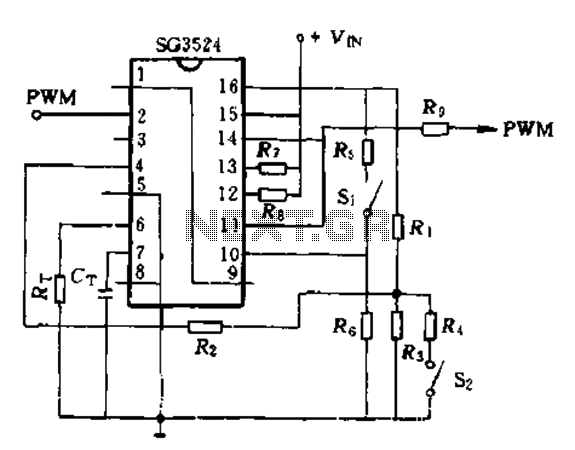
Dedicated PWM ICs integrate precision timing circuits, error amplifiers, and output drivers into a single package. The TL494 and SG3525 are classic examples featuring:
- Adjustable frequency (1 kHz to 300 kHz) via external RC networks
- Push-pull or single-ended output configurations
- Dead-time control to prevent shoot-through in bridge circuits
The duty cycle (D) is determined by comparing a sawtooth waveform (Vramp) with a control voltage (Vctrl):
Modern PWM Modules: Digital vs. Hybrid
Contemporary modules like the MAX1556 (digital) and LT6992 (hybrid) combine analog precision with digital programmability. Key advancements include:
- I2C/SPI interfaces for dynamic frequency and duty cycle adjustment
- Integrated MOSFET drivers with 4A peak current capability
- Spread-spectrum modulation for EMI reduction
Case Study: Digital PWM Resolution
For a 16-bit PWM running at 1 MHz, the time resolution (Δt) is:
Thermal and Power Considerations
High-frequency operation (≥500 kHz) requires careful thermal management. Power dissipation in a PWM driver with RDS(on) = 50 mΩ and IRMS = 3A is:
Application-Specific PWM ICs
Specialized variants address niche requirements:
- Motor Control: DRV8323 integrates three-phase gate drivers with current sensing
- LED Drivers: TLC59731 provides 12-bit grayscale PWM with auto-temperature derating
- RF Applications: ADF4351 combines PLL with 12-bit PWM for agile frequency synthesis
Noise and Jitter Performance
High-end PWM generators like the Si8261 achieve jitter below 50 ps RMS by using:
- Differential clock inputs with LVDS signaling
- On-chip voltage-controlled delay lines (VCDLs)
- Sub-micron CMOS processes with guard-ring isolation
2.3 Analog PWM Generation Techniques
Analog PWM generation relies on continuous-time signal processing to modulate the duty cycle of a pulse train in response to an input voltage. Unlike digital methods, which rely on discrete-time counters and comparators, analog techniques exploit the natural behavior of operational amplifiers, comparators, and nonlinear feedback loops to produce a PWM signal with high resolution and minimal quantization noise.
Core Principle: Triangle Wave Modulation
The most common analog PWM method involves comparing a modulating signal (typically an audio or control voltage) with a high-frequency triangle or sawtooth carrier wave. The intersection points between these signals determine the switching instants, translating the input amplitude into a proportional duty cycle.
where D(t) is the instantaneous duty cycle, Vin(t) is the input signal, and Vmin, Vmax define the carrier's peak-to-peak range. The triangle wave's linearity directly impacts PWM distortion, with nonlinearities introducing harmonic artifacts.
Circuit Implementation: Op-Amp Based Generators
A classic implementation uses an integrator to generate the triangle wave and a comparator for modulation:
- Integrator Stage: An op-amp with capacitive feedback converts a square wave into a triangle wave via constant-current charging/discharging. The time constant Ï„ = RC sets the carrier frequency.
- Comparator Stage: A high-speed comparator (e.g., LM311) switches when the triangle wave crosses the input signal, producing a PWM output. Hysteresis may be added to suppress chatter.
Nonlinear Effects and Compensation
Real-world integrators exhibit slew rate limiting and capacitor dielectric absorption, distorting the triangle wave. Compensation techniques include:
- Slew Rate Enhancement: Adding a feedforward path with a small resistor in series with the integrator capacitor.
- Dead-Time Control: Introducing deliberate delay in the comparator to prevent shoot-through in power stages.
where β is the feedback factor accounting for nonlinearities.
Advanced Techniques: Voltage-to-Frequency Conversion
For applications requiring variable frequency alongside duty cycle modulation (e.g., resonant converters), voltage-controlled oscillators (VCOs) like the 4046 PLL IC generate a carrier whose frequency is proportional to Vin. The resulting PWM spectrum becomes adaptive, reducing EMI in sensitive applications.
Practical Considerations
- Noise Immunity: Analog PWM is susceptible to ground bounce and supply noise. Differential signaling or guard rings improve robustness.
- Thermal Drift: Comparator offsets and integrator time constants vary with temperature. Auto-zeroing circuits or precision references mitigate drift.
3. PWM Generation Using Embedded Software
3.1 PWM Generation Using Embedded Software
Fundamentals of Software-Based PWM
Pulse-width modulation (PWM) generation via embedded software relies on precise timing control through microcontroller peripherals such as timers and compare registers. The duty cycle D is defined as the ratio of the pulse width ton to the total period T:
Modern microcontrollers implement PWM through hardware-assisted software control, where timer interrupts or direct memory access (DMA) updates duty cycle values stored in capture/compare registers. The resolution of the PWM signal is determined by the counter register's bit depth:
Implementation Strategies
Two primary methods exist for software PWM generation:
- Timer Interrupt Method: Uses periodic interrupts to toggle GPIO pins based on a precomputed duty cycle table. This approach is flexible but consumes CPU cycles.
- Hardware Timer PWM Mode: Leverages dedicated timer peripherals with auto-reload and compare features, offloading the PWM generation entirely to hardware.
Timer Interrupt Method
For microcontrollers without dedicated PWM hardware, a timer interrupt service routine (ISR) can manually set and clear output pins. The ISR must:
- Increment a counter variable
- Compare the counter against the desired duty cycle value
- Set the output high when counter ≤ duty value
- Clear the output when counter > duty value
- Reset the counter at the period boundary
// Example ARM Cortex-M timer ISR for PWM generation
void TIM2_IRQHandler(void) {
   static uint16_t pwm_counter = 0;
   pwm_counter++;

   if (pwm_counter <= duty_cycle) {
      GPIO_SetPin(PWM_OUTPUT_PIN);
   } else {
      GPIO_ClearPin(PWM_OUTPUT_PIN);
   }

   if (pwm_counter >= PWM_PERIOD) {
      pwm_counter = 0;
   }

   TIM_ClearFlag(TIM2, TIM_FLAG_Update);
}
Hardware-Assisted PWM
Modern microcontrollers like STM32 or ESP32 provide dedicated PWM timer blocks that only require software initialization:
- Configure timer clock source and prescaler
- Set auto-reload register (ARR) for period
- Set capture/compare register (CCR) for duty cycle
- Enable PWM output mode on GPIO
- Start the timer
// STM32 HAL library PWM initialization
TIM_HandleTypeDef htim;
TIM_OC_InitTypeDef sConfigOC;

htim.Instance = TIM1;
htim.Init.Prescaler = 0;
htim.Init.CounterMode = TIM_COUNTERMODE_UP;
htim.Init.Period = 999; // 1kHz PWM with 1MHz clock
htim.Init.ClockDivision = TIM_CLOCKDIVISION_DIV1;
HAL_TIM_PWM_Init(&htim);

sConfigOC.OCMode = TIM_OCMODE_PWM1;
sConfigOC.Pulse = 250; // 25% duty cycle
sConfigOC.OCPolarity = TIM_OCPOLARITY_HIGH;
sConfigOC.OCFastMode = TIM_OCFAST_DISABLE;
HAL_TIM_PWM_ConfigChannel(&htim, &sConfigOC, TIM_CHANNEL_1);

HAL_TIM_PWM_Start(&htim, TIM_CHANNEL_1);
Advanced Techniques
For high-resolution PWM, consider these optimizations:
- Dithering: Modulate duty cycle between adjacent values to achieve sub-LSB resolution
- Phase-Shifted PWM: Multiple timers generate interleaved signals for reduced ripple
- DMA-Based Updates: Stream duty cycle values from memory without CPU intervention
The maximum achievable PWM frequency is constrained by both the timer clock speed and the required resolution:
For example, a 72MHz clock with 16-bit resolution yields a maximum frequency of approximately 1.1kHz while maintaining full resolution. Higher frequencies require either reduced resolution or advanced prescaling techniques.
3.2 Algorithmic Approaches to PWM
Mathematical Basis of PWM Generation
Pulse-width modulation (PWM) generation relies on precise timing control, where the duty cycle D is defined as the ratio of the pulse duration Ton to the total period T:
For a desired output voltage Vout with a supply voltage VDC, the duty cycle is derived as:
This linear relationship forms the foundation of most PWM algorithms, where precise control of D enables accurate voltage or power regulation.
Counter-Based PWM Algorithms
Digital PWM generation often employs a counter-comparator approach. A free-running N-bit counter increments at a clock frequency fclk, producing a sawtooth waveform. The PWM period T is determined by:
A comparator triggers the output transition when the counter matches a duty cycle register value Dreg. This method is widely used in microcontrollers and FPGA-based systems due to its deterministic timing and low computational overhead.
Delta-Sigma Modulation for High-Resolution PWM
When higher resolution is required than native counter bits allow, delta-sigma modulation can be employed. This technique uses noise shaping to push quantization error to higher frequencies, achieving effective resolutions beyond hardware limitations. The first-order delta-sigma modulator follows:
where x[n] is the input signal and y[n] is the PWM output. This approach is particularly effective in audio amplification and precision motor control applications.
Space Vector PWM for Three-Phase Systems
In three-phase inverters, space vector PWM (SVPWM) provides superior DC bus utilization compared to sinusoidal PWM. The algorithm:
- Transforms three-phase voltages to α-β coordinates
- Determines the sector in the space vector hexagon
- Calculates dwell times for adjacent active vectors and zero vectors
The voltage vector Vref is synthesized using:
where T1 and T2 are the dwell times for vectors V1 and V2, and Ts is the switching period.
Predictive PWM Control
Model predictive control (MPC) algorithms optimize PWM generation by evaluating future system states. The cost function:
minimizes tracking error x* - x while penalizing control effort Δu, with prediction horizon Np and weighting matrices Q, R. This approach provides fast dynamic response in power electronic converters.
Hardware Implementation Considerations
When implementing PWM algorithms in hardware, several factors must be considered:
- Dead-time compensation: Necessary to prevent shoot-through in bridge circuits
- Switching frequency limitations: Determined by device thermal constraints
- Quantization effects: Finite register width impacts minimum pulse width
- Interrupt latency: Critical for software-based implementations
3.3 Simulation of PWM in Software Environments
Mathematical Foundation of PWM Simulation
Simulating pulse-width modulation (PWM) in software requires a precise mathematical representation of the signal. The PWM waveform is characterized by its duty cycle D, period T, and amplitude A. The duty cycle is defined as the ratio of the pulse width Ï„ to the period:
In discrete-time simulation, the PWM signal is sampled at a frequency fs, where fs must be significantly higher than the PWM frequency fPWM = 1/T to avoid aliasing. The Nyquist criterion mandates:
However, in practice, a sampling rate of at least 10fPWM is recommended to accurately capture the rising and falling edges of the PWM signal.
Software Tools for PWM Simulation
Several software environments are commonly used for PWM simulation, each with unique advantages:
- SPICE-based simulators (LTspice, PSpice): Provide accurate transient analysis of PWM-driven circuits, including non-ideal effects like rise/fall times and parasitic elements.
- MATLAB/Simulink: Offers block-based modeling of PWM systems with extensive control system libraries.
- Python (SciPy, NumPy, matplotlib): Enables custom PWM simulation with full control over the mathematical model and visualization.
- LabVIEW: Useful for real-time PWM simulation and hardware-in-the-loop testing.
Implementation in MATLAB/Simulink
In Simulink, PWM generation can be implemented using the Pulse Generator block or through a custom comparator-based approach. The comparator method compares a modulating signal (e.g., sine wave) with a high-frequency carrier (typically triangular):
The following Simulink blocks are essential for accurate PWM simulation:
- Repeating Sequence (for carrier generation)
- Relational Operator (for comparison)
- Switch (for output conditioning)
Python Implementation Example
For discrete-time simulation in Python, the PWM signal can be generated using NumPy and visualized with matplotlib:
import numpy as np
import matplotlib.pyplot as plt

# Parameters
f_pwm = 1e3      # PWM frequency (Hz)
f_s = 100e3      # Sampling frequency (Hz)
D = 0.75         # Duty cycle (0 to 1)
T = 1 / f_pwm    # Period (s)
t = np.arange(0, 2*T, 1/f_s)  # Time vector

# Generate PWM signal
pwm_signal = np.where(np.mod(t, T) < D * T, 1, 0)

# Plot
plt.plot(t, pwm_signal)
plt.xlabel('Time (s)')
plt.ylabel('Amplitude')
plt.title('Simulated PWM Signal (D=0.75)')
plt.grid(True)
plt.show()
Practical Considerations
When simulating PWM in software, the following factors must be accounted for:
- Numerical stability: High-frequency PWM signals may require adaptive time-stepping in differential equation solvers.
- Computational efficiency: Vectorized operations (e.g., in NumPy) significantly speed up large-scale simulations.
- Non-ideal effects: Dead-time, switching delays, and parasitic capacitance/inductance can be modeled for higher fidelity.
Validation Against Analytical Models
The simulated PWM output should be validated against the theoretical Fourier series representation of an ideal PWM signal:
Harmonic distortion analysis (e.g., THD calculation) can be performed using FFT-based methods to verify simulation accuracy.
4. Sinusoidal PWM (SPWM)
4.1 Sinusoidal PWM (SPWM)
Sinusoidal Pulse Width Modulation (SPWM) is a modulation technique used to generate a quasi-sinusoidal output from a DC source by controlling the duty cycle of a high-frequency carrier signal. Unlike regular PWM, which produces a square wave, SPWM approximates a sine wave by varying the pulse width in proportion to the amplitude of a reference sine wave.
Mathematical Foundation
The fundamental principle of SPWM involves comparing a high-frequency triangular carrier wave (Vcarrier) with a low-frequency sinusoidal reference wave (Vref). The intersection points determine the switching instants of the PWM signal. The modulation index (ma) is defined as:
where:
- Vref is the peak amplitude of the reference sine wave,
- Vcarrier is the peak amplitude of the triangular carrier wave.
The output voltage (Vout) of an inverter using SPWM can be expressed in terms of the DC bus voltage (VDC) and modulation index:
Generation Method
SPWM is typically implemented using the following steps:
- Carrier Wave Selection: A triangular wave with frequency fc (carrier frequency) is generated, usually at several kHz to minimize harmonic distortion.
- Reference Sine Wave: A sinusoidal wave with the desired output frequency fo (e.g., 50 Hz or 60 Hz) is generated.
- Comparator Operation: The PWM signal switches high when Vref > Vcarrier and low otherwise.
Harmonic Analysis
SPWM reduces lower-order harmonics compared to square-wave modulation. The harmonic spectrum consists of sidebands centered around multiples of the carrier frequency. The dominant harmonics occur at:
where k and l are integers. Proper selection of fc ensures harmonics are pushed to higher frequencies, making them easier to filter.
Practical Implementation
SPWM is widely used in:
- Inverters: For AC motor drives and renewable energy systems.
- Uninterruptible Power Supplies (UPS): To generate clean sinusoidal output.
- Audio Amplifiers: Class-D amplifiers use SPWM for high-efficiency audio signal reproduction.
Microcontrollers and dedicated PWM controllers (e.g., TI’s C2000 series, STM32) often include hardware support for SPWM generation, reducing computational overhead.
Limitations and Improvements
While SPWM is effective, it has limitations:
- Voltage Utilization: The maximum fundamental output voltage is limited to VDC/2.
- Third-Harmonic Injection: Adding a third harmonic to the reference signal increases voltage utilization without distortion.
- Space Vector PWM (SVPWM): An advanced method that offers better DC bus utilization and lower harmonics.
4.2 Space Vector PWM (SVPWM)
Space Vector PWM (SVPWM) is an advanced modulation technique used in three-phase inverters to generate PWM signals that optimize voltage utilization and minimize harmonic distortion. Unlike sinusoidal PWM, SVPWM treats the inverter as a single entity, synthesizing the desired output voltage vector by combining the eight possible switching states of a three-phase inverter.
Mathematical Foundation
The three-phase voltages can be represented as space vectors in the α-β plane using the Clarke transformation:
This transformation converts the three-phase quantities into a two-dimensional orthogonal reference frame. The resulting space vector Vref is synthesized using the adjacent active vectors and zero vectors.
Switching States and Voltage Vectors
A three-phase inverter has eight possible switching states (six active and two zero), each corresponding to a unique voltage vector in the α-β plane:
- Active vectors (V1 to V6): Correspond to non-zero output voltages, spaced 60° apart.
- Zero vectors (V0, V7): Correspond to all upper or lower switches being ON, resulting in zero output voltage.
The reference vector Vref is approximated by switching between the two nearest active vectors and zero vectors over a PWM period.
Duty Cycle Calculation
The dwell times for the active vectors are calculated based on the sector in which Vref lies. For a reference vector in Sector 1:
where Ts is the switching period, Vdc is the DC bus voltage, and θ is the angle of Vref within the sector.
Implementation Steps
- Determine the sector: Calculate the angle of Vref and identify the sector (1 to 6).
- Compute dwell times: Use the above equations to find T1, T2, and T0.
- Generate switching sequence: Apply the active and zero vectors in a symmetric sequence (e.g., V0-V1-V2-V7-V2-V1-V0) to minimize switching losses.
Advantages Over Sinusoidal PWM
- Higher DC bus utilization: SVPWM achieves a 15.47% higher fundamental voltage magnitude compared to sinusoidal PWM.
- Reduced harmonic distortion: The optimized switching sequence lowers total harmonic distortion (THD).
- Better dynamic response: The vector-based approach allows faster control in motor drives and grid-tied inverters.
Practical Applications
SVPWM is widely used in:
- AC motor drives (induction and PMSM)
- Grid-connected inverters for renewable energy systems
- Uninterruptible power supplies (UPS)
Dead-Time Insertion in PWM Signals
Dead-time insertion is a critical technique in PWM-driven power electronics to prevent shoot-through currents in half-bridge or full-bridge configurations. When two complementary PWM signals drive high-side and low-side switches, a finite delay must be introduced between their transitions to ensure one switch is fully off before the other turns on.
Mathematical Basis of Dead-Time Calculation
The required dead time (tdead) depends on the turn-off delay (toff) and turn-on delay (ton) of the power switches (e.g., MOSFETs or IGBTs). For a conservative estimate, the dead time must satisfy:
where tmargin is an additional safety margin (typically 10-20% of the worst-case delay). For example, if a MOSFET has toff,max = 100 ns and ton,min = 50 ns, with tmargin = 20 ns, the minimum dead time becomes:
Implementation Methods
Dead-time insertion can be implemented in hardware or software:
- Hardware: Dedicated dead-time generator ICs (e.g., LM5050) or RC-based delay circuits introduce fixed delays between complementary signals.
- Software: Microcontrollers or FPGAs programmatically insert delays in PWM generation logic. For example, STM32 microcontrollers use the Advanced Timer (TIM1/TIM8) dead-time registers (DTG[7:0]) to configure dead time as:
where Tclk is the timer clock period.
Impact on PWM Linearity
Dead-time insertion introduces non-linearity in the output voltage, especially at low duty cycles. The effective duty cycle (Deff) deviates from the commanded duty cycle (D) by:
where TPWM is the PWM period, and sgn(Iload) accounts for current direction. This distortion is compensated using dead-time compensation algorithms in motor drives and inverters.
Practical Considerations
- Switching Frequency: Dead time becomes a larger fraction of the PWM period at high frequencies, reducing effective voltage resolution.
- Parasitic Capacitance: MOSFET gate-drain capacitance (Cgd) can inadvertently couple signals, requiring additional dead time.
- Thermal Effects: Delays vary with temperature, necessitating adaptive dead-time control in high-reliability systems.
5. Noise and EMI Considerations
5.1 Noise and EMI Considerations
Fundamental Noise Mechanisms in PWM
PWM signals inherently generate high-frequency spectral content due to their abrupt transitions between logic levels. The Fourier series representation of an ideal PWM waveform with duty cycle D and period T reveals harmonic components at integer multiples of the switching frequency fsw:
The harmonic amplitudes follow a sinc function envelope, with nulls occurring at integer multiples of 1/D. Practical implementations exhibit additional spectral contamination from:
- Rise/fall time imperfections (typically 1-10ns for power MOSFETs)
- Ground bounce effects (ΔV ≈ Lloop di/dt)
- Parasitic LC resonances in PCB traces
EMI Coupling Pathways
PWM-related interference propagates through three primary mechanisms:
Conducted emissions dominate below 30MHz, with characteristic impedance mismatches causing standing waves. Radiated emissions peak at frequencies where PCB trace lengths approach λ/4 of harmonic components.
Mitigation Techniques
Time-Domain Strategies
- Controlled edge rates: Optimal trade-off between switching losses and EMI achieved when:
$$ t_r = \frac{0.35}{f_{max}} $$where fmax is the highest frequency of concern
- Dead-time optimization: Prevents shoot-through while minimizing voltage spikes
Frequency-Domain Approaches
Spread spectrum techniques modulate fsw with triangular or Hershey-kiss profiles, reducing peak emissions by 10-15dB. The modulation depth Δf should satisfy:
where Tmeas is the EMI receiver's integration time.
Layout Considerations
Critical PCB design rules for PWM circuits:
| Parameter | Recommended Value |
|---|---|
| Loop area | < 4cm2 per amp of switched current |
| Ground plane cutouts | Minimum 3× dielectric thickness from high dv/dt nodes |
| Via stitching | λ/20 spacing at highest harmonic frequency |
Differential-mode noise dominates below 1MHz, while common-mode becomes significant at higher frequencies due to parasitic capacitances (typically 2-10pF in power stages).
Filter Design Methodology
A second-order LC filter with damping factor ζ = 0.707 provides optimal attenuation:
Practical implementations often require additional stages for broadband suppression, with ferrite beads effective above 10MHz for impedance matching.
5.2 Heat Dissipation and Power Handling
Thermal Dynamics in PWM-Driven Systems
PWM-driven power electronics, such as MOSFETs and IGBTs, generate heat primarily due to conduction and switching losses. The total power dissipation Pdiss in a switching device can be decomposed into:
where Pcond represents conduction losses and Psw accounts for switching losses. Conduction losses arise from the device's on-state resistance RDS(on) and the RMS current IRMS:
Switching Losses and Frequency Dependence
Switching losses occur during the transient phases of turn-on and turn-off. For a MOSFET switching at frequency fsw, the energy dissipated per cycle Esw is given by:
where tr and tf are the rise and fall times, respectively. The total switching power loss scales linearly with frequency:
Thermal Resistance and Junction Temperature
The device's junction temperature Tj must be kept below its maximum rated value to prevent failure. The thermal path from junction to ambient is characterized by thermal resistance θJA:
where Ta is the ambient temperature. For high-power applications, a heatsink with low thermal resistance θHS is often necessary to maintain safe operating conditions.
Practical Design Considerations
- Parasitic Inductance: Stray inductance in the switching loop increases voltage spikes and switching losses.
- Gate Drive Strength: Faster switching reduces Esw but may increase EMI.
- Thermal Interface Materials: Thermal pads or compounds minimize θJC (junction-to-case resistance).
Case Study: Buck Converter Thermal Analysis
Consider a synchronous buck converter with Vin = 24V, Vout = 5V, Iout = 10A, and fsw = 500kHz. Using a MOSFET with RDS(on) = 5mΩ and tr = tf = 20ns, the conduction and switching losses are:
For θJA = 40°C/W and Ta = 25°C, the junction temperature reaches:
This exceeds typical limits (125°C), necessitating a heatsink or reduced switching frequency.
5.3 Optimization of PWM Parameters for Efficiency
Trade-offs in Duty Cycle and Frequency Selection
The efficiency of a PWM-driven system depends critically on the interplay between duty cycle (D) and switching frequency (fsw). For a resistive load, power dissipation due to switching losses scales quadratically with frequency:
where C is the parasitic capacitance of the switching node. Conversely, conduction losses (Pcond) rise with duty cycle due to I2R effects. The optimal operating point minimizes total losses:
Dead-Time Optimization
In bridge converters, dead time (td) prevents shoot-through but introduces cross-conduction losses. The optimal dead time balances:
- Transistor turn-off delays (toff)
- Diode reverse recovery charge (Qrr)
- Gate driver propagation delay
For a MOSFET-based H-bridge, the empirical formula for minimum dead time is:
Harmonic Distortion Mitigation
High-frequency PWM reduces audible noise but increases EMI. The harmonic content of a PWM signal follows a sinc envelope:
where n is the harmonic order. For motor drives, frequencies above 20 kHz avoid audible effects, while RF applications may require spread-spectrum modulation techniques.
Thermal Considerations
Switching devices exhibit a thermal impedance (Zth) that limits maximum fsw. The junction temperature rise is:
For forced-air cooling, derating curves typically show a 10% efficiency drop per 25°C above 100°C ambient.
Case Study: Buck Converter Optimization
A 12V-to-5V buck converter with L = 10 µH and Coss = 100 pF achieves peak efficiency (94%) at:
- D = 0.42 (accounting for diode forward voltage)
- fsw = 500 kHz (trade-off between inductor size and FET losses)
- td = 30 ns (calibrated via oscilloscope measurements)
6. Key Books and Publications on PWM
6.1 Key Books and Publications on PWM
- PDF The Common Use of Pulse Width Modulation "PWM" Technique in ... - IJSR — PWM signal . 2.1 PWM Generation . Several methods were used to Generate PWM signals. one of them Analogue method. Analogue PWM signals (comparator output) can be made by combining a saw- tooth waveform and a sinusoid, the higher the DC level is, the wider the PWM pulses are. The DC level is the demand
- Power Electronic Converters - Wiley Online Library — Power Electronic Converters PWM Strategies and Current Control Techniques Edited by ... A CIP record for this book is available from the British Library ISBN 978-1-84821-195-7 ... 1.5. Generation of PWM signals ..... 13 1.5.1. Reverse sawtooth wave.....
- Pulse width modulation for power converters : principles and practice ... — Preface -- Acknowledgments -- Nomenclature -- Chapter 1: Introduction to Power Electronic Converters -- 1.1 Basic Converter Topologies -- 1.2 Voltage Source/Stiff Inverters -- 1.3 Switching Function Representation of Three-Phase Converters -- 1.4 Output Voltage Control -- 1.5 Current Source/Stiff Inverters -- 1.6 Concept of a Space Vector -- 1. ...
- Power Electronic Converters: PWM Strategies and Current Control ... — A voltage converter changes the voltage of an electrical power source and is usually combined with other components to create a power supply. This title is devoted to the control of static converters, which deals with pulse-width modulation (PWM) techniques, and also discusses methods for current control. Various application cases are treated. The book is ideal for professionals in power ...
- PDF Chapter 2 Pulse-Width Modulation - IFORAP — turbation. A small-signal model can be obtained for the modulator by computing the component in the PWM output at the frequency of the sinusoidal perturbation. Such small-signal models will be developed in Sect. 2.3 for both constant-frequency and variable-frequency PWM. For AC-DC and DC-AC converters, the reference signal typically contains at
- C2000 ePWM Developer's Guide - Texas Instruments — The enhanced pulse width modulator (ePWM) peripheral is a key element in controlling many of the power electronic systems found in both industrial and automotive applications. C2000™ real-time microcontrollers offer many differentiated features within the ePWM peripheral that allow for advanced control techniques. This
- PDF 101 Pulse-width modulation - Massachusetts Institute of Technology — PWM PWM control Duty 95% 50% 5% cycle Supply voltage Load A simple comparator with a sawtooth carrier can turn a sinusoidal command into a pulse-width modulated output. In general, the larger the command signal, the wider the pulse. Pulse-width modulation The output of a PWM amplifier is either zero or tied to the supply voltage, holding losses ...
- PDF The Design of A High Frequency Pulse Width Modulation Integrated ... — The Pulse Width Modulation (PWM) has been playing an active role in circuits and systems for many years. The PWM is an irreplaceable part of the switch-mode power supplies (SMPS) and the class D power amplifiers (PA). The high frequency PWM operation is the key for having more compact SMPSs and class D PAs since it provides
- PDF Analog Pulse Width Modulation U1B VREF - Texas Instruments — of the input signal (V IN). The average output voltage (V O) depends on the amplitude of the PWM waveform (V PWM) which is typically determined by the supply voltages of the comparator. (2) Because the supply voltage of the comparator directly impacts the output voltage, PWM circuits without feedback have no power supply rejection.
- (PDF) PWM techniques: Introduction - Academia.edu — the circuits become huge and complex [2] . This paper presents a new technique to generate the PWM signal by analyzing the data using the software before transferring to the binary file. The binary file is then programmed onto the ROM such that each bit represents the data of the PWM signal.
6.2 Online Resources and Tutorials
- Power Electronic Converters : PWM Strategies and Current Control ... — Generation of PWM signals 13 1.6. Determination of the reference waves varef k, vbref k, and vcref k from the reference waves varef k, vbref k, vcref k 24 1.7. Conclusion 32 1.8. Bibliography 33; Chapter 2. Space Vector Modulation Strategies 35 Nicolas PATIN and Vincent LANFRANCHI 2.1. Inverters and space vector PWM 35 2.2.
- Explain PAM, PWM and PPM generation with relevant waveforms. - Ques10 — This signal is then applied to an inverting amplifier to amplify its signal level to have the demodulated output with almost equal amplitude with the modulating signal. Generation of PWM. PWM signal can be generated by using a comparator, where modulating signal and sawtooth signal form the input of the comparator.
- C2000 ePWM Developer's Guide - Texas Instruments — UP-DOWN. The frequency of the PWM events (F. PW M) is controlled by the time-base period (TBPRD) register and the mode of the time-base counter. For up and down count modes: T. PWM = TB PR D + 1 T. TBCLK (1) F. PW M = 1 TPW M (2) For up-down count mode: T. PWM = 2*TB PRD*T. TBCLK (3) F. PW M = 1 TPW M (4) Where, T. PWM. is the period of the PWM ...
- PWM Generator Simulink MATLAB — It serves as the source of the periodic signal in PWM generation. 3.2 Comparator Block. The Comparator block compares the generated square wave with a reference signal, typically a sinusoidal wave or a sawtooth wave. ... In power electronics, PWM is employed for controlling the power flow in devices like inverters and switching power supplies ...
- FPGA based PWM generation - Tutorials - Digilent Forum — FPGA's can do some really neat things when it comes to PWM generation that micro-controllers can't do. Specifically, because they can operate at such high speeds, they can toggle the analog output line in unique fashions, and at *much* higher frequencies, than most PWM controllers. ... Another way of saying this is that the bit-reversed PWM ...
- (PDF) PWM techniques: Introduction - Academia.edu — the circuits become huge and complex [2] . This paper presents a new technique to generate the PWM signal by analyzing the data using the software before transferring to the binary file. The binary file is then programmed onto the ROM such that each bit represents the data of the PWM signal.
- PDF Multichannel PWM TPU Function (MCPWM) - NXP Semiconductors — The multichannel PWM function uses two channels that are externally gated (using single EOR gates) together to form a single PWM signal. This allows a full 0% to 100% duty cycle range under a much wider range of TPU operating conditions than other PWM functions. The MCPWM function can operate in edge-aligned (EA) mode or in center-aligned (CA ...
- GitHub - sanampudig/iiitb_pwm_gen — Contribute to sanampudig/iiitb_pwm_gen development by creating an account on GitHub. ... Pulse Width Modulation is a famous technique used to create modulated electronic pulses of the desired width. The duty cycle is the ratio of how long that PWM signal stays at the high position to the total time period. ... This PWM generator generates 10Mhz ...
- PDF Analog Pulse Width Modulation U1B VREF - Texas Instruments — Many PWM circuits operate without the comparator included in the feedback loop of an amplifier. For these circuits, the output duty cycle is a function of the amplitude of the triangle wave (V TRI) and amplitude of the input signal (V IN). The average output voltage (V O) depends on the amplitude of the PWM waveform (V PWM
- TL594 Pulse-Width-Modulation Control Circuit - Texas Instruments — 1• Complete PWM Power-Control Circuitry • Uncommitted Outputs for 200-mA Sink or Source Current • Output Control Selects Single-Ended or Push-Pull Operation • Internal Circuitry Prohibits Double Pulse at Either Output • Variable Dead Time Provides Control Over Total Range • Internal Regulator Provides a Stable 5-V Reference Supply ...
6.3 Research Papers and Case Studies
- EEE - 6 - ICS - 6.3 - Generation and Demodulation of PAM PPM and PWM ... — EEE_6_ICS_6.3_generation-and-demodulation-of-PAM-PPM-and-PWM-with-waveforms - Free download as PDF File (.pdf), Text File (.txt) or read online for free. The document discusses the generation and demodulation of PAM, PPM, and PWM signals. It explains that PAM encodes information by varying the amplitude of pulses, with the pulse amplitude proportional to the modulating signal.
- PDF Power Electronic Converters. PWM Strategies and ... - Semantic Scholar — Chapter 7. Electromagnetic Compatibility of Variable Speed Drives: Impact of PWM Control Strategies 159 Bertrand REVOL 7.1. Introduction 159 7.2. Objectives of an EMC study 161 7.3. EMC mechanisms in static converters 162 7.4. Time-domain simulation 167 7.5. Frequency-domain modeling: a tool for the engineer 169 7.6. PWM control 178 7.7.
- Matlab/Simulink Implementation and Analysis of Three Pulse-width ... — Academia.edu is a platform for academics to share research papers. MATLAB/SIMULINK IMPLEMENTATION AND ANALYSIS OF THREE PULSE-WIDTH-MODULATION (PWM) TECHNIQUES ... (PD) PWM scheme enables generation of the most excellent output voltage among the three PWM schemes. ... [17]: 2 1 Van = √ sin(ω t) + sin(3ω t) 6 3 2 1 Vbn = √ sin(ω t − 2π ...
- Design and Analysis of DC-DC PWM Converter and DC-AC Converter — Fig 3.1.2 Signal Generation Circuit ... the switching frequency becomes twice and voltage amplitude is reduced to half in case of unipolar PWM. ... This paper presents a unique feed-forward Space ...
- (PDF) PWM techniques: Introduction - Academia.edu — This is the most preferred method since PWM offers many advantages. In this dissertation, the applications of PWM techniques on different types of power electronic converters are studied. The simulation is carried out using SIMULINK and MULTISIM. In the first part of this paper, the generations of PWM signal using different methods are explained.
- PDF Design and Analysis of Various Inverters Using Different Pwm ... - Theijes — which can suite for all applications. As per the advanced technology in solid state power electronic devices and microprocessors, various pulse-width modulation (PWM) techniques have been developed for different industrial applications. For the above reasons, the PWM techniques have been the subject of intensive research since 1970s.
- Advanced PWM Strategies for Complicated Topologies — For phase-a, Fig. 6.37 shows a typical case of 180° interleaving for two paralleled inverters in one switching cycle, where the reference signal is compared with the carriers to generate the PWM signals. It can be seen that the two inverters share the same reference voltage, but the carrier of inverter 2 is shifted 180° with respect to that ...
- Comparison of the EMI performance of LED PWM dimming techniques for LED ... — Pulse Width Modulation (PWM) can be used to generate or modify sinusoidal wave [1,2] to control [3], modify characteristics of a generator [4,5], actuate and adjust induction motors [6,3 ...
- PDF Design and Implementation of Switched Mode Power Supply Using Pwm Concepts — MOSFET switch, driven by PWM feedback signal, to control the output voltage level. An Isolation Transformer is used to isolate the DC output from input supply. The transformer output is again rectified by the high frequency Diode bridge rectifier and is filtered using a capacitor to give the regulated DC output.
- (PDF) Model Predictive Controller-based, Single Phase ... - ResearchGate — This research article discusses a Model Predictive Control(MPC) based, digital control strategy for single-phase Pulse Width Modulated (PWM) voltage source inverters, used in Uninterrupted Power ...