
Solar Panel Optimizing Battery Charger
The solar panel circuit described operates under a dynamic environment, where the efficiency of energy conversion is paramount. The V-I curve indicates the relationship between voltage and current, essential for understanding the panel's performance across different lighting conditions. The transition region of the curve is critical, as it represents the maximum power point (MPP), which is the optimal operating condition for energy extraction.
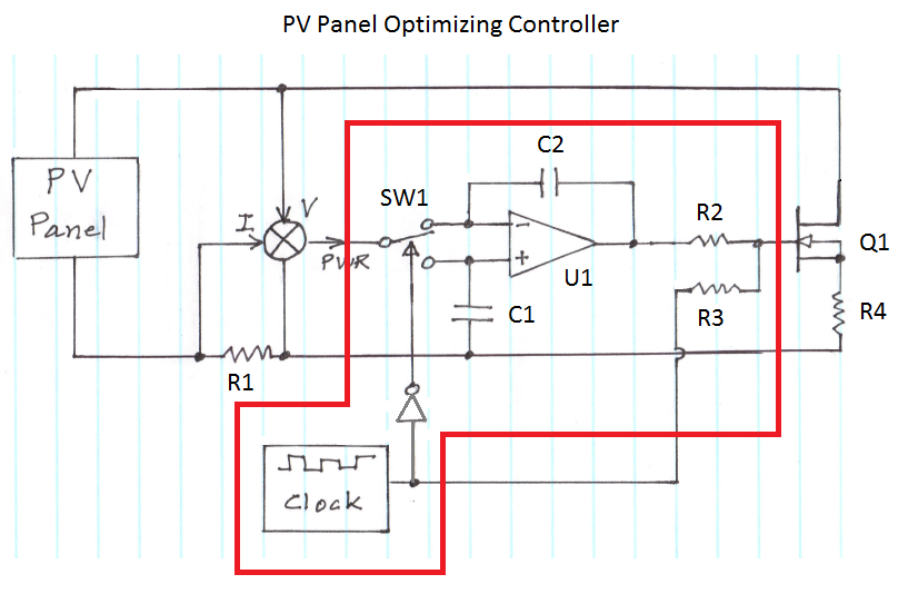
In practical applications, battery chargers integrated with maximum power point tracking (MPPT) algorithms are employed to maximize energy capture from solar panels. These chargers utilize switching regulators that adjust load conditions to ensure the panel operates at or near the MPP. The feedback mechanism involves monitoring the output power and modulating the load accordingly. When the panel is underperforming due to lower light levels, the system can reduce the load to increase voltage, thereby enhancing power delivery.
The power monitoring circuit, featuring resistor R1 and a multiplier, plays a vital role in providing real-time feedback on the power output. This feedback is essential for the MPPT controller to make informed adjustments to the load, ensuring optimal energy utilization. The implementation of the SPICE simulation allows for the evaluation of different operational scenarios, providing insights into the panel's behavior under varying conditions.
The design considerations for such a system include the selection of components that can handle the expected current ranges, the implementation of efficient switching techniques, and the calibration of the monitoring circuit to ensure accurate power readings. Overall, the integration of these elements contributes to the development of a robust solar energy harvesting system capable of adapting to fluctuating environmental conditions while maintaining high efficiency in energy conversion and storage.Figure shows the V-I curve for a typical solar panel (Sharp ND-224U1F), and output power under different lighting conditions. The solar panel behaves like a constant current source at high current, and like a voltage source at low current.
The transition region is where the highest power can be obtained. The voltage and particularly the current at the optimum point vary considerably with the amount of light incident to the panel. The solar panel is typically used to charge batteries since solar energy is only available during the day, but typical electrical power usage extends during dark periods. On cloudy days, limited power may be available even at mid-day. Therefore, an optimized battery charger must be able to determine the "maximum power point" (MPP) of the panel under the current condition and adjust the load to match it, keeping in mind that the MPP varies during the day as a function of the amount of available light and the panel`s temperature.
Fortunately, switching regulators of the type used in high efficiency battery chargers can vary the load while maintaining the proper output voltage for battery charging. It continuously monitors the panel`s output power while modulating the load by a small amount. When the power increases as the load is increased, the controller increases the average load. When the power does not change between the two load values, the panel is operating across the MPP. See figure 2 below. In the figure above, points P1 and P2 correspond to non-optimized operation. The current is high, but the delivered power is less than it would be if the load was a little lighter (less current and more voltage).
When the charger operates between points P1 and P2, the unequal power levels drive the controller to a lower average load (lower current) in order to increase the delivered power. Eventually, the operating points move to P3/P4, where the power delivered is equal and the controller stays at that level, until the amount of light or the temperature (or the battery state of charge) change.
In that figure, points P1 and P2 (respectively P3/P4) are more widely spaced than desirable, for illustration. If the points were so widely spaced, the controller would never operate at the peak power. You can see that P3 and P4 are about 5W below the MPP. By making the modulation a small fraction of the available power, points P3/P4 will move much closer together and the controller will operate very close to the MPP.
The charger provides the load. In our example, the modulation represents about 5% of the average load. This amount can be adjusted depending on the power of the actual panel used, the sensitivity and dynamic range of the power monitoring circuit and how close you want to be from the MPP. Typical values will be around a few percent. The Power Monitor around R1 and the multiplier delivers a voltage that represents the power delivered by the panel under the current conditions of light, temperature and load.
Aside from an obvious scaling factor (this model is operated with current from 0. 5 to 1A, the Sharp panel is rated at almost 9A at full illumination), the curves match the shape of those on the Sharp datasheet fairly well. Different illuminations can be represented by varying the current source I1. In that simulation, the current source I1 is stepped through 3 different values using the SPICE. STEP directive. To do this, just add the following text as a single line in the file "standard. dio" under the library folder in the installation directory of LT Spice, "C:Program FilesLTCLTspiceIVlibcmp" on this computer: This model is probably grossly inacurate with regard to actual performance, particularly regarding the power avai
🔗 External reference
Related Circuits
The basic clock circuit is similar to the binary clock and uses 7 ICs to produce the 20 digital bits for 12 hour time, plus AM and PM. A standard watch crystal oscillator (32,768) is used as the time...
The Vx2SE is a simple discrete voltage-doubling SE for driving an LED. If the load is a red or green LED, J1 is used together with just one red or green LED for threshold detection (no 1381). For driving...
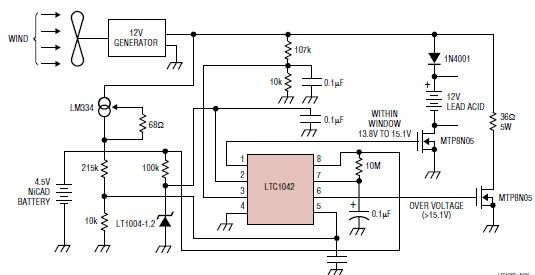
This simple wind charger circuit project is designed using the LTC1042 monolithic CMOS window comparator, manufactured by Linear Technology. The wind charger circuit utilizes wind power to generate the energy necessary for charging Ni-Cd or lead-acid batteries. When the...
This file is copyrighted. The individual who uploaded this work and first used it in licensing holds the rights. The provided information indicates that the file is protected by copyright, with the rights belonging to the individual who initially uploaded...
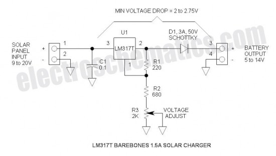
This is a simple and cost-effective solar battery charger that can be constructed by hobbyists. It has some limitations compared to other similar controllers, but it also provides several benefits. While primarily designed for charging lead-acid batteries, it can...
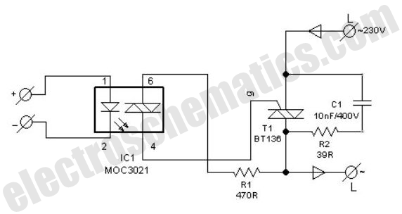
Modern power control systems utilize electronic devices such as Thyristors for power switching, phase control, and chopper applications. These devices also find applications in various other areas. Thyristors are semiconductor devices that act as switches, allowing control over high-voltage and...
Warning: include(partials/cookie-banner.php): Failed to open stream: Permission denied in /var/www/html/nextgr/view-circuit.php on line 713
Warning: include(): Failed opening 'partials/cookie-banner.php' for inclusion (include_path='.:/usr/share/php') in /var/www/html/nextgr/view-circuit.php on line 713