
PSPICE Examples for EE-201

The described circuit analysis procedure encompasses a variety of analytical techniques to derive key electrical characteristics of a circuit. The process begins with the computation of gain and resistances, which are essential for understanding circuit performance. The Transfer Function dialog box allows users to define how input signals are transformed into output signals, facilitating the evaluation of both the voltage gain and input/output resistances.
For Thevenin's equivalent circuit analysis, the removal of the load resistor and the substitution with a high-value resistor ensures that the circuit operates correctly under simulation constraints. The introduction of a VIEWPOINT at node 4 provides a visual representation of the open-circuit voltage, which is crucial for calculating Thevenin's voltage.
The DC Sweep Analysis enhances the simulation's capability by systematically varying an input parameter and analyzing the corresponding output. This method is particularly beneficial for identifying how changes in input voltage affect the circuit's performance metrics, including the output voltage and current through specific components.
The use of the IPRINT and VPRINT2 commands ensures that the relevant data is logged for further analysis. By setting the DC values to include in the output file, a comprehensive record of the circuit's performance across the defined input range is maintained.
The amplifier circuit modeled by a current-controlled current source demonstrates the influence of varying input voltage on output voltage, with the resistance changes providing insight into the circuit's stability and response characteristics. The Parametric Sweep feature allows for dynamic analysis of resistor values, showcasing how component variations impact overall circuit behavior.
Finally, the AC Analysis setup provides a framework for frequency response evaluation, essential for understanding circuit performance under alternating current conditions. By selecting specific frequencies and sweep parameters, users can obtain a detailed frequency response, which is critical for applications in signal processing and communications. Overall, this comprehensive approach to circuit analysis enables engineers to optimize circuit designs and predict performance accurately.Computes the gain and the input and output resistances and automatically sends the results to the output file. To specify the transfer function, choose Setup from the Analysis menu and open the Transfer Function dialog box.
In the Output Variable box specify the output voltage, and in the Input Source box type the input source name. The transfer f unction analysis can be used conveniently to obtain the Thevenin`s equivalent circuit. The use of this analysis to obtain the Thevenin`s equivalent circuit is demonstrated in the following example We want to obtain the Thevenin`s equivalent circuit with respect to the 3. 5 W resistor. The 3. 5 W resistor is replaced by an open circuit. Since in PSpice two or more elements must be connected to each node, the 3. 5 W resistor is replaced by an infinitely high value resistor as shown. A VIEWPOINT is added at node 4 to display the open-circuit voltage (Thevenin`s voltage). To obtain the output or Thevenin`s resistance, the transfer Function is enabled. In the Output variable box we type V(4), and in the Input Source box, we type V1. DC voltage or current sources may be swept over a range through the use of the DC Sweep Analysis. The DC Sweep is similar to the node voltage analysis, but adds more flexibility. In the DC sweep, the input variable is varied over a range of values. For each value of the input variable, the DC operating point is computed. If the transfer function is also enabled the small-signal DC gain and the input/output resistances are also computed.
For the circuit shown print and plot the voltage V23, IR2, and IR3 as the input voltage is varied from 0 to 100 V in 5 V increment. Select the Setup from the analysis menu, click the DC Sweep dialog button. The DC Sweep dialog box appears. For the Sweep Variable type select the voltage source, and set its name to V1. Using the Sweep type linear, specify the starting value, end value and increment. IPRINT and VPRINT2 are inserted in the appropriate locations to send the desired currents and voltages to the output file.
To include the DC values double click on each print icon and set the DC = to yes. The circuit shown below represents an amplifier circuit modeled by a current-controlled current source. The input voltage is varied from 0 to 1. 5 V with an increment of 0. 25 V. The resistance Re changes by ± 25%. Plot the DC transfer characteristic output voltage V4 versus the input voltageV1 for each value of the resistance Re.
Select the Setup from the analysis menu, click the DC Sweep dialog button. The DC Sweep dialog box appears. For the Sweep Variable type select the voltage source, and set its name to V1. Using the Sweep type linear, specify the starting value, end value and increment (0, 0. 25, and 1. 5). The Parametric Sweep can be used to change the value of the resistor Re. To do this, get a part called PARAM from Special. slb and place it in your circuit. Double click on the text PARAMETERS. The attributes allow you to define up to three different variable parameters. For NAME1= define a parameter, say Rval, and for VALUE1= set an initial value of 250. Click the OK button to accept the attribute. We must now change the value of Re to the name of the parameter. Double click on the value of R1 and in place of its value type in the text {Rval}. Next select the Analysis and then Setup and click the Parametric button. Mark Global Parameter, set Name to Rval. Under Sweep Type, mark Value List and set the Values: to 187. 5 250 312. 5. Perform the simulation. To run an AC Analysis, we require an AC source with AC specifications such VSRC, ISRC or VAC and IAC. In the Analysis setup dialog box, click on the AC sweep button. Complete the AC Sweep and Noise Analysis box as required. For AC analysis at a single frequency say 60 Hz, select Linear AC Sweep, set Total Pts: to 1, Start Freq: to 60, and End freq: to 60.
For frequency response over a wide range of frequencies 🔗 External reference
Related Circuits
Digital filters are powerful yet user-friendly, contributing to the popularity of digital signal processing (DSP). For example, a low-pass filter with a cutoff frequency of 1 kHz can be implemented in analog electronics. This method is often utilized for...
Examples of an OFDM modulation system. The graph illustrates the input data signal (.... --- Ol01100) and the data signal by the string. The input signal is separated into components such as "00", "ll", "10", "00", "01", and other...

The UGN3113U is an open collector Hall effect integrated circuit (IC) switch designed for use in position sensing applications. The circuit includes a current limiting feature that utilizes a crystal capacitor, along with resistors R1 and R2, to manage...
A collection of drawings showcasing various applications of the 555 timer IC. These include schematic diagrams sourced from online resources and literature, intended for personal reference. The original web pages from which these schematics were derived have not been...
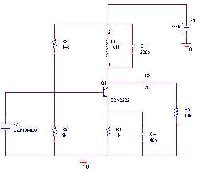
A simulation of a 27 MHz transmitter circuit is to be conducted using PSPICE. The circuit diagram is provided as Figure 1 in the following content. The 27 MHz transmitter circuit typically consists of several key components, including an oscillator,...

Input J4 features an offset function that is activated only when no plug is inserted into J4, as the switching contact of J4 connects to the positive supply voltage through the protection resistor R8. The inverting sum of all...